Mijn Formule Test
Mijn Testpagina
Panorama
Numerieke Differentiatie Formules
Numerieke Integratie Formules
Closed Newton–Cotes Formulae
Degree |
Common name |
Formula |
Error term
|
1 |
Trapezoid rule |
![{\displaystyle {\frac {b-a}{2}}(f_{0}+f_{1})}](https://wikimedia.org/api/rest_v1/media/math/render/svg/898874be93dd6abb959fcbef070b3ddcb08c96f9) |
|
2 |
Simpson's rule |
![{\displaystyle {\frac {b-a}{6}}(f_{0}+4f_{1}+f_{2})}](https://wikimedia.org/api/rest_v1/media/math/render/svg/d80da787700ee8d6df4377f5b2108594c8063f0f) |
|
3 |
Simpson's 3/8 rule |
![{\displaystyle {\frac {b-a}{8}}(f_{0}+3f_{1}+3f_{2}+f_{3})}](https://wikimedia.org/api/rest_v1/media/math/render/svg/576acf1c9916f415bcdc06ede2876e3687ab8776) |
|
4 |
Boole's rule |
![{\displaystyle {\frac {b-a}{90}}(7f_{0}+32f_{1}+12f_{2}+32f_{3}+7f_{4})}](https://wikimedia.org/api/rest_v1/media/math/render/svg/5c0825d67febc5a0f8529b0cff79c65691119a32) |
|
Closed Newton–Cotes Formulae
Degree |
Common name |
Formula |
Error term
|
1 |
Trapezoid rule |
![{\displaystyle {\frac {h}{2}}(f_{0}+f_{1})}](https://wikimedia.org/api/rest_v1/media/math/render/svg/190810541a767e7404bb18a6ad65e7b27e928d0c) |
|
2 |
Simpson's rule |
![{\displaystyle {\frac {h}{3}}(f_{0}+4f_{1}+f_{2})}](https://wikimedia.org/api/rest_v1/media/math/render/svg/8cea0ac47e190b2b8c49d0e198becf0e6e1ff2ee) |
|
3 |
Simpson's 3/8 rule |
![{\displaystyle {\frac {3h}{8}}(f_{0}+3f_{1}+3f_{2}+f_{3})}](https://wikimedia.org/api/rest_v1/media/math/render/svg/5b934c3efd3938691b589460ffdba3c57af5926f) |
|
4 |
Boole's rule |
![{\displaystyle {\frac {2h}{45}}(7f_{0}+32f_{1}+12f_{2}+32f_{3}+7f_{4})}](https://wikimedia.org/api/rest_v1/media/math/render/svg/a86158a4ee409ea52d1f989cac7d5d1744907635) |
|
Closed Newton–Cotes Formulae
Degree |
Common name |
Formula |
Error term
|
1 |
Trapezoid rule |
![{\displaystyle {\frac {1}{2}}h(f_{0}+f_{1})}](https://wikimedia.org/api/rest_v1/media/math/render/svg/68de05480cb2883e853d9255980549917620a79b) |
|
2 |
Simpson's rule |
![{\displaystyle {\frac {1}{3}}h(f_{0}+4f_{1}+f_{2})}](https://wikimedia.org/api/rest_v1/media/math/render/svg/4a4e9dec2f81c97bfc44a1e58c23e6f35abe5a87) |
|
3 |
Simpson's 3/8 rule |
![{\displaystyle {\frac {3}{8}}h(f_{0}+3f_{1}+3f_{2}+f_{3})}](https://wikimedia.org/api/rest_v1/media/math/render/svg/8ed026d5b0eed1f5a3f10ee553704938083d36c1) |
|
4 |
Boole's rule |
![{\displaystyle {\frac {2}{45}}h(7f_{0}+32f_{1}+12f_{2}+32f_{3}+7f_{4})}](https://wikimedia.org/api/rest_v1/media/math/render/svg/88ee4b456cd042c9c36fe608b9e4a36a6323f84b) |
|
![{\displaystyle V={\begin{bmatrix}1&\alpha _{1}&\alpha _{1}^{2}&\dots &\alpha _{1}^{n-1}\\1&\alpha _{2}&\alpha _{2}^{2}&\dots &\alpha _{2}^{n-1}\\1&\alpha _{3}&\alpha _{3}^{2}&\dots &\alpha _{3}^{n-1}\\\vdots &\vdots &\vdots &\ddots &\vdots \\1&\alpha _{m}&\alpha _{m}^{2}&\dots &\alpha _{m}^{n-1}\end{bmatrix}}}](https://wikimedia.org/api/rest_v1/media/math/render/svg/693d72fcd6a92174e05ca765729a6a705a51f284)
![{\displaystyle V_{n}={\begin{bmatrix}x_{1}&x_{2}&\cdots &x_{n}\\x_{1}^{2}&x_{2}^{2}&\cdots &x_{n}^{2}\\\vdots &\vdots &\ddots &\vdots \\x_{1}^{n}&x_{2}^{n}&\cdots &x_{n}^{n}\end{bmatrix}}}](https://wikimedia.org/api/rest_v1/media/math/render/svg/97d3d04c816320a552ef3ebe3939cc9612d0ce21)
![{\displaystyle V={\begin{bmatrix}0^{0}&0^{1}&0^{2}&\dots &0^{n}\\1^{0}&1^{1}&1^{2}&\dots &1^{n}\\2^{0}&2^{1}&2^{2}&\dots &2^{n}\\\vdots &\vdots &\vdots &\ddots &\vdots \\n^{0}&n^{1}&n^{2}&\dots &n^{n}\end{bmatrix}}}](https://wikimedia.org/api/rest_v1/media/math/render/svg/fae209b0711f3202ee33e880dbe1254c827c208e)
![{\displaystyle f(x)=\sum _{n=0}^{\infty }{\frac {f^{(n)}(x_{0})}{n!}}(x-x_{0})^{n}.}](https://wikimedia.org/api/rest_v1/media/math/render/svg/486489130b09506da5cdbd244635ce46b7d782f4)
![{\displaystyle {\begin{bmatrix}f_{0}\\f_{1}\\f_{2}\\\vdots \\f_{n}\end{bmatrix}}={\begin{bmatrix}0^{0}&0^{1}&0^{2}&\dots &0^{n}\\1^{0}&1^{1}&1^{2}&\dots &1^{n}\\2^{0}&2^{1}&2^{2}&\dots &2^{n}\\\vdots &\vdots &\vdots &\ddots &\vdots \\n^{0}&n^{1}&n^{2}&\dots &n^{n}\end{bmatrix}}{\begin{bmatrix}{\frac {f^{(0)}(x_{0})}{0!}}h^{0}\\{\frac {f^{(1)}(x_{0})}{1!}}h^{1}\\{\frac {f^{(2)}(x_{0})}{2!}}h^{2}\\\vdots \\{\frac {f^{(n)}(x_{0})}{n!}}h^{n}\end{bmatrix}}\Rightarrow {\begin{bmatrix}f^{(0)}(x_{0}){\frac {h^{0}}{0!}}\\f^{(1)}(x_{0}){\frac {h^{1}}{1!}}\\f^{(2)}(x_{0}){\frac {h^{2}}{2!}}\\\vdots \\f^{(n)}(x_{0}){\frac {h^{n}}{n!}}\end{bmatrix}}={\begin{bmatrix}0^{0}&0^{1}&0^{2}&\dots &0^{n}\\1^{0}&1^{1}&1^{2}&\dots &1^{n}\\2^{0}&2^{1}&2^{2}&\dots &2^{n}\\\vdots &\vdots &\vdots &\ddots &\vdots \\n^{0}&n^{1}&n^{2}&\dots &n^{n}\end{bmatrix}}^{-1}{\begin{bmatrix}f_{0}\\f_{1}\\f_{2}\\\vdots \\f_{n}\end{bmatrix}}}](https://wikimedia.org/api/rest_v1/media/math/render/svg/02fba1a5854f3a35410c58f85924b24918f605b0)
![{\displaystyle {\begin{bmatrix}{\frac {1}{1!}}&{\frac {1}{2!}}&{\frac {1}{3!}}&\dots &{\frac {1}{n!}}\\0&{\frac {1}{1!}}&{\frac {1}{2!}}&\dots &{\frac {1}{(n-1)!}}\\0&0&{\frac {1}{1!}}&\dots &{\frac {1}{(n-2)!}}\\\vdots &\vdots &\vdots &\ddots &\vdots \\0&0&0&\dots &{\frac {1}{1!}}\end{bmatrix}}^{-1}\!\!\!\!=\,{\begin{bmatrix}{\frac {B_{0}}{0!}}&{\frac {B_{1}}{1!}}&{\frac {B_{2}}{2!}}&\dots &{\frac {B_{n-1}}{(n-1)!}}\\0&{\frac {B_{0}}{0!}}&{\frac {B_{1}}{1!}}&\dots &{\frac {B_{n-2}}{(n-2)!}}\\0&0&{\frac {B_{0}}{0!}}&\dots &{\frac {B_{n-3}}{(n-3)!}}\\\vdots &\vdots &\vdots &\ddots &\vdots \\0&0&0&\dots &{\frac {B_{0}}{0!}}\end{bmatrix}}}](https://wikimedia.org/api/rest_v1/media/math/render/svg/8fa6a25a2e62ea52b9327915dbb3719f15f1df05)
Constructing the interpolation polynomial
edit
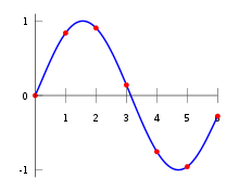
The red dots denote the data points (xk,yk), while the blue curve shows the interpolation polynomial.
Suppose that the interpolation polynomial is in the form
-
The statement that p interpolates the data points means that
-
If we substitute equation (1) in here, we get a system of linear equations in the coefficients . The system in matrix-vector form reads
-
We have to solve this system for to construct the interpolant The matrix on the left is commonly referred to as a Vandermonde matrix.
-
-
of Lagrange basis polynomials
-