Hello!
My interest in editing Wikipedia is in illustrating articles, so let me know if you wish some article on science, mathematics or technology illustrated.
Here is some of my work to date; click on images for more details:
Templates edit
Template:venn3 edit
{{venn3
|caption=Breakdown of British and<br>American [[traffic collision]] causes
|unit=%
|labelA=Driver factors
|labelB=Roadway<br>factors
|labelC=Vehicle factors
|countA=57
|countB=3
|countC=2
|countAB=27
|countAC=6
|countBC=1
|countABC=3
}}
Template:bartable edit
| Element | Percent by mass | Atomic percent (calc.) | ||
|---|---|---|---|---|
| Oxygen | 65% | 25.6% | ||
| Carbon | 18% | 9.5% | ||
| Hydrogen | 10% | 63% | ||
| Nitrogen | 3% | 1.3% | ||
| Calcium | 1.5% | 0.24% | ||
| Phosphorus | 1.2% | 0.24% | ||
| Potassium | 0.2% | 0.03% | ||
| Sulfur | 0.2% | 0.04% | ||
| Chlorine | 0.2% | 0.04% | ||
| Sodium | 0.1% | 0.03% | ||
| Magnesium | 0.05% | 0.01% | ||
| Iron | 3 g in men, 2.3 g in women | |||
| Cobalt, Copper, Zinc, Iodine | < 0.05% each | |||
| Selenium, Fluorine | < 0.01% each | |||
Template:stereo image edit
| Stereo image | |||
|---|---|---|---|
| |||
| |||
| |||
| |||
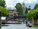
| The Church of the Holy Sepulchre (Round Church) and the south end of Round Church Street in Cambridge, England. | |||

-
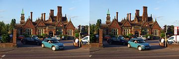
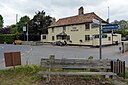
 The Jenny Wren pub and bus stop with an approaching Citi 1 bus.
 -
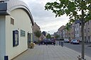
 The Golden Hind pub.
 -
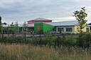
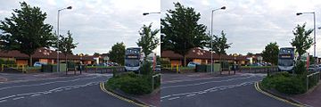 The Grove primary school at King's Hedges, Cambridge.
 -
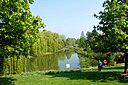
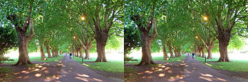 Avenue of London plane trees on Jesus Green, Cambridge, England.
 -
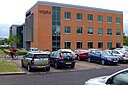
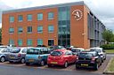
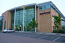
 Autonomy building at Cambridge Business Park.
 -
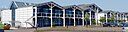
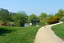
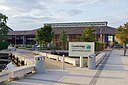
 Cambridge Leisure Park.
 -
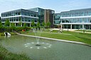
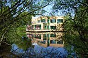
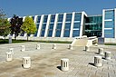
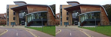 University of Cambridge's Faculty of Education's Donald McIntyre Building.
 -
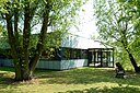
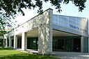
 The Cavendish Building at Homerton College's present site.


Images edit
Original drawings edit
3D render edit


Pseudo-3D SVG edit
-
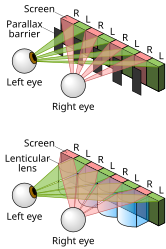 ☎∈ Comparison of parallax-barrier and lenticular autostereoscopic displays. Note: The figure is not to scale.
 -
 ☎∈ Golomb rulers in interior design: Example of a conference room with proportions of a Golomb ruler, making it configurable to 10 different sizes.
 -
-

-

-
-

-
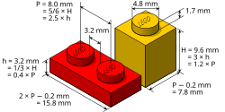
 ☎∈ Some 3D shapes in isometric projection. Black labels denote dimensions of the 3D object, while red labels denote dimensions of the 2D projection (drawing).
 -
 ☎∈ Massing model showing the shape of the Bank of China Tower. The labels correspond to the number of 'X' shapes on each outward facing side.
 -

-

-
-
-
 ☎∈ Visualisation of composition by volume of Earth's atmosphere. Data is from NASA Langley: http://www.nasa.gov/centers/langley/pdf/245893main_MeteorologyTeacherRes-Ch2.r4.pdf .
 -
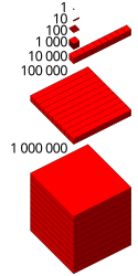
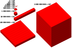
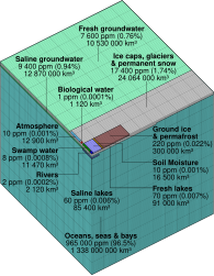 ☎∈ Visualisation of the distribution (by volume) of water on Earth. Each tiny cube (such as the one representing biological water) corresponds to approximately 1000 cubic km of water, with a mass of approximately 1 trillion tonnes (200000 times that of the Great Pyramid of Giza or 5 times that of Lake Kariba, arguably the heaviest man-made object). The entire block comprises 1 million tiny cubes. Data is from http://ga.water.usgs.gov/edu/waterdistribution.html .


Charts edit
-
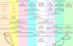
 ☎∈ Timeline of the colleges of the University of Cambridge in the order their students are presented for graduation, compared with some events in British history.
 -
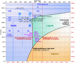 ☎∈ Log-lin pressure-temperature phase diagram of water. The Roman numerals indicate various ice phases.
 -
![☎∈ Comparison of sizes of semiconductor manufacturing process nodes with some microscopic objects and visible light wavelengths. At this scale, the width of a human hair is about 10 times that of the image.[1]](//upload.wikimedia.org/wikipedia/commons/thumb/c/c7/Comparison_semiconductor_process_nodes.svg/250px-Comparison_semiconductor_process_nodes.svg.png) ☎∈ Comparison of sizes of semiconductor manufacturing process nodes with some microscopic objects and visible light wavelengths. At this scale, the width of a human hair is about 10 times that of the image.[1]
☎∈ Comparison of sizes of semiconductor manufacturing process nodes with some microscopic objects and visible light wavelengths. At this scale, the width of a human hair is about 10 times that of the image.[1] -
![☎∈ Comparison of the 1962 US Standard Atmosphere graph of geometric altitude against air density, pressure, the speed of sound and temperature with approximate altitudes of various objects.[2]](//upload.wikimedia.org/wikipedia/commons/thumb/9/9d/Comparison_US_standard_atmosphere_1962.svg/202px-Comparison_US_standard_atmosphere_1962.svg.png) ☎∈ Comparison of the 1962 US Standard Atmosphere graph of geometric altitude against air density, pressure, the speed of sound and temperature with approximate altitudes of various objects.[2]
☎∈ Comparison of the 1962 US Standard Atmosphere graph of geometric altitude against air density, pressure, the speed of sound and temperature with approximate altitudes of various objects.[2] -
-
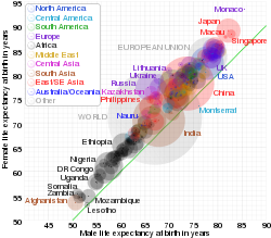
![☎∈ Graphs of life expectancy at birth for some sub-Saharan countries showing the fall in the 1990s primarily due to the AIDS pandemic.[3]](//upload.wikimedia.org/wikipedia/commons/thumb/4/41/Comparison_subsaharan_life_expectancy.svg/187px-Comparison_subsaharan_life_expectancy.svg.png)
-
![☎∈ Estimated and projected populations of the world and its inhabited continents from 1950 to 2100. The shaded regions correspond to range of projections by the United Nations Department of Economic and Social Affairs; for example, it estimates that the world population will reach 8 billion between 2022 and 2035.[4]](//upload.wikimedia.org/wikipedia/commons/thumb/4/43/UN_DESA_continent_population_1950_to_2100.svg/250px-UN_DESA_continent_population_1950_to_2100.svg.png) ☎∈ Estimated and projected populations of the world and its inhabited continents from 1950 to 2100. The shaded regions correspond to range of projections by the United Nations Department of Economic and Social Affairs; for example, it estimates that the world population will reach 8 billion between 2022 and 2035.[4]
☎∈ Estimated and projected populations of the world and its inhabited continents from 1950 to 2100. The shaded regions correspond to range of projections by the United Nations Department of Economic and Social Affairs; for example, it estimates that the world population will reach 8 billion between 2022 and 2035.[4] -
![☎∈ Proportion of world (countries with data) nominal GDP for the countries with the top 10 highest nominal GDP in 2010, from 1980 to 2010 with IMF projections until 2016. Countries marked with an asterisk are non-G8 countries. Grey lines show actual US dollar values.[5]](//upload.wikimedia.org/wikipedia/commons/thumb/1/14/Historical_top_10_nominal_GDP_proportion.svg/250px-Historical_top_10_nominal_GDP_proportion.svg.png)
-
![☎∈ Plot of Voyager 2's heliocentric velocity against its distance from the sun, illustrating the use of gravity assist to accelerate the spacecraft by Jupiter, Saturn and Uranus. To observe Triton, Voyager 2 passed over Neptune's north pole resulting in an acceleration out of the plane of the ecliptic and reduced velocity away from the sun.[6]](//upload.wikimedia.org/wikipedia/commons/thumb/2/2c/Voyager_2_velocity_vs_distance_from_sun.svg/250px-Voyager_2_velocity_vs_distance_from_sun.svg.png) ☎∈ Plot of Voyager 2's heliocentric velocity against its distance from the sun, illustrating the use of gravity assist to accelerate the spacecraft by Jupiter, Saturn and Uranus. To observe Triton, Voyager 2 passed over Neptune's north pole resulting in an acceleration out of the plane of the ecliptic and reduced velocity away from the sun.[6]
☎∈ Plot of Voyager 2's heliocentric velocity against its distance from the sun, illustrating the use of gravity assist to accelerate the spacecraft by Jupiter, Saturn and Uranus. To observe Triton, Voyager 2 passed over Neptune's north pole resulting in an acceleration out of the plane of the ecliptic and reduced velocity away from the sun.[6] -
![☎∈ Inferred orbits of 6 stars around supermassive black hole candidate Sagittarius A* at the Milky Way galactic centre.[7]](//upload.wikimedia.org/wikipedia/commons/thumb/c/c1/Galactic_centre_orbits.svg/208px-Galactic_centre_orbits.svg.png) ☎∈ Inferred orbits of 6 stars around supermassive black hole candidate Sagittarius A* at the Milky Way galactic centre.[7]
☎∈ Inferred orbits of 6 stars around supermassive black hole candidate Sagittarius A* at the Milky Way galactic centre.[7] -

-

-
-


![☎∈ Comparison of sizes of semiconductor manufacturing process nodes with some microscopic objects and visible light wavelengths. At this scale, the width of a human hair is about 10 times that of the image.[1]](/wiki/File:Comparison_semiconductor_process_nodes.svg)
![☎∈ Comparison of the 1962 US Standard Atmosphere graph of geometric altitude against air density, pressure, the speed of sound and temperature with approximate altitudes of various objects.[2]](/wiki/File:Comparison_US_standard_atmosphere_1962.svg)

![☎∈ Graphs of life expectancy at birth for some sub-Saharan countries showing the fall in the 1990s primarily due to the AIDS pandemic.[3]](/wiki/File:Comparison_subsaharan_life_expectancy.svg)
![☎∈ Estimated and projected populations of the world and its inhabited continents from 1950 to 2100. The shaded regions correspond to range of projections by the United Nations Department of Economic and Social Affairs; for example, it estimates that the world population will reach 8 billion between 2022 and 2035.[4]](/wiki/File:UN_DESA_continent_population_1950_to_2100.svg)
![☎∈ Proportion of world (countries with data) nominal GDP for the countries with the top 10 highest nominal GDP in 2010, from 1980 to 2010 with IMF projections until 2016. Countries marked with an asterisk are non-G8 countries. Grey lines show actual US dollar values.[5]](/wiki/File:Historical_top_10_nominal_GDP_proportion.svg)
![☎∈ Plot of Voyager 2's heliocentric velocity against its distance from the sun, illustrating the use of gravity assist to accelerate the spacecraft by Jupiter, Saturn and Uranus. To observe Triton, Voyager 2 passed over Neptune's north pole resulting in an acceleration out of the plane of the ecliptic and reduced velocity away from the sun.[6]](/wiki/File:Voyager_2_velocity_vs_distance_from_sun.svg)
![☎∈ Inferred orbits of 6 stars around supermassive black hole candidate Sagittarius A* at the Milky Way galactic centre.[7]](/wiki/File:Galactic_centre_orbits.svg)


Other original drawings edit
-
 ☎∈ Trajectories of projectiles launched at different elevation angles but the same speed of 10 m/s in a vacuum and uniform downward gravity field of 10 m/s2. Points are at 0.05 s intervals and length of their tails is linearly proportional to their speed. t = time from launch, T = time of flight, R = range and H = highest point of trajectory (indicated with arrows).
 -
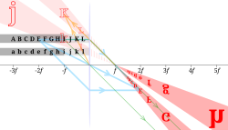 ☎∈ Images of the black letters in an ideal convex lens of focal length f are shown in red. Selected rays are shown for letters E, I and K in blue, green and orange, respectively. Note that E (at 2f) has an equal-size, real and inverted image; I (at f) has its image at infinity; and K (at f/2) has a double-size, virtual and upright image.
 -
-
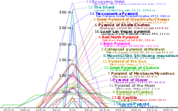 ☎∈ Comparison of approximate profiles of some pyramidal or near-pyramidal buildings. Where the base is an oblong, the longer side is shown. Dotted lines indicate original heights, where data is available.
 -
![☎∈ Development of the Petronas Towers Tower 1 level 43 floor plan from a Rub el Hizb symbol.[8]](//upload.wikimedia.org/wikipedia/commons/thumb/7/7b/Petronas_Towers_level_43_plan.svg/83px-Petronas_Towers_level_43_plan.svg.png)
-
-
-
-

-
-
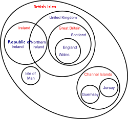
 ☎∈ Five-set Venn diagram using congruent ellipses in a radially symmetrical arrangement devised by Branko Grünbaum. Labels have been simplified for greater readability; for example, A denotes A ∩ Bc ∩ Cc ∩ Dc ∩ Ec (or A ∩ ~B ∩ ~C ∩ ~D ∩ ~E), while BCE denotes Ac ∩ B ∩ C ∩ Dc ∩ E (or ~A ∩ B ∩ C ∩ ~D ∩ E).
 -
 ☎∈ Euler diagram of some types of quadrilaterals. (UK) denotes British English and (US) denotes American English.
 -
 ☎∈ Euler diagram of types of triangles, assuming isosceles triangles have at least 2 equal sides, implying that equilateral triangles are also isosceles triangles.
 -
-
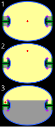
 ☎∈
☎∈
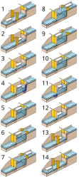
Comparison of a knock-out with and without trapping, and overprinting for perfect and imperfect registration. Rows are as follows:Knock-out
without trappingKnock-out
with trappingOverprinting
1. The cyan (lighter) plate,
2. The magenta (darker) plate,
3. Result with perfect registration (some monitors show slight misalignment), and
4. Result with imperfect registration. -

-
-

-

-
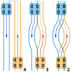 ☎∈ Illustration of 4-rail, 3-rail and 2-rail funicular railway layouts (note the gaps in the rails, and the unconventional wheels in the 2-rail layout).
 -
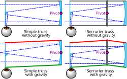 ☎∈Principle of operation of a Serrurier truss for a telescope compared to a simple truss. For clarity, only the top and bottom structural elements are shown. Red and green lines denote elements under tension and compression, respectively.
 -
-

-
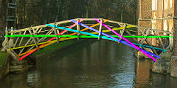 ☎∈ The tangent and radial trussing of the Mathematical Bridge in Queens' College, Cambridge, with its tangential members highlighted.
 -
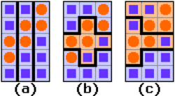 ☎∈ How Gerrymandering can influence electoral results on a non-proportional system.
Example for a state with 3 equally sized districts, 15 voters and 2 parties: Plum (squares) and Orange (circles).
In (a), creating 3 mixed-type districts yields a 3–0 win to Plum — a disproportional result considering the state-wide 9:6 Plum majority.
In (b), Orange wins the urban district while Plum wins the rural districts — the 2-1 result reflects the state-wide vote ratio.
In (c), gerrymandering techniques ensure a 2-1 win to the state-wide minority Orange party.


![☎∈ Development of the Petronas Towers Tower 1 level 43 floor plan from a Rub el Hizb symbol.[8]](/wiki/File:Petronas_Towers_level_43_plan.svg)


Processed images edit
SVG with embedded bitmap, designed to be easily translated into different languages edit
-
-

-
 ☎∈ Location of all successful soft landings on the Moon to date. Dates are landing dates in UTC.(Uses embedded bitmaps as icons.)
 -
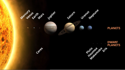 ☎∈ Planets and dwarf planets of the Solar System. Sizes are to scale, but relative distances from the Sun are not. (Uses 4 bitmaps of different shapes and rotated text.)
 -
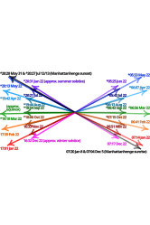 ☎∈ Manhattanhenge map of Manhattan Island, New York City (latitude approximately 40° N) centered on the intersection of Park Avenue and 34th Street, with times and directions of sunsets (solid line) and sunrises (dotted line) in 2011. Times marked with "*" have been adjusted for daylight saving. The purple, pink and green arrows correspond approximately to the summer solstice, equinoxes and winter solstice, respectively.
 -
![☎∈ Fukushima I and II nuclear accidents overview map showing evacuation and other zone progression and selected radiation levels. (Uses gradients and more complex shapes.)]]](//upload.wikimedia.org/wikipedia/commons/thumb/b/bc/Fukushima_accidents_overview_map.svg/187px-Fukushima_accidents_overview_map.svg.png)
-
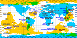 ☎∈ Cities and towns which are near antipodes in equirectangular projection. Blue labels correspond to the cyan areas and brown labels correspond to the yellow areas. Areas where blue and yellow overlap (coloured green) are land antipodes
 -

-

-

-

-
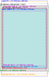
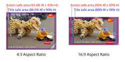 ☎∈ Illustration of Action Safe and Title Safe areas for 4:3 and 16:9 aspect ratios according to the BBC. (Uses multiple instances of one bitmap.)
 -
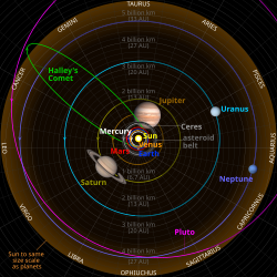 ☎∈ Orbits and directions of travel of the planets, Pluto, Ceres and Halley's Comet, viewed perpendicular to the ecliptic directly above the Sun. Their positions correspond to their configuration during the 5–6 June 2012 transit of Venus. Constellation names correspond to constellations on the ecliptic in the given directions. In the full SVG image, brighter parts of orbits are nearer to the viewer than the ecliptic and darker parts are farther. Planets' sizes are to scale and distances are roughly to (a different) scale. (Uses stroke-dashoffset and stroke-dasharray to shade parts of ellipses.)
 -


![☎∈ Fukushima I and II nuclear accidents overview map showing evacuation and other zone progression and selected radiation levels. (Uses gradients and more complex shapes.)]]](/wiki/File:Fukushima_accidents_overview_map.svg)


Other processed images edit
-
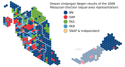
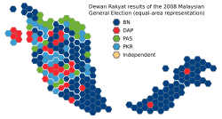 ☎∈ Results of the Malaysian Dewan Rakyat based on the 2008 general election, showing parliamentary constituencies represented by equal-area hexagons with approximate geographic locations.
 -
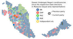
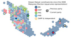 ☎∈ Current composition of the Malaysian Dewan Rakyat with changes since the 2008 general election emphasized for clarity. The parliamentary constituencies are represented by equal-area hexagons, positioned according to approximate geographic locations.
 -
-
-
-
 ☎∈ Aerial view of the Fukushima I plant area before the accidents. When this photograph was taken in 1975, Unit 6 was under construction.
 -
 ☎∈ Locations of large artificial objects on the Moon superimposed on data from the Clementine (spacecraft) mission in [[equirectangular projection.
 -
-
-

-

-
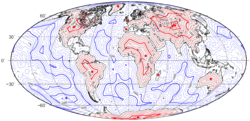 ☎∈ Mollweide projection map of distance to the nearest coastline (including oceanic islands, but not lakes) with red spots marking the poles of inaccessibility of main land masses, Britain, and the Iberian Peninsula. Thin isolines are 250 km apart; thick lines 1000 km.
 -
-
![☎∈ A television set drawn in near-isometric pixel art (left) compared with the same image with isometric proportions (right), enlarged to show the pixel structure.[9]](//upload.wikimedia.org/wikipedia/commons/b/bf/Pixelart-tv-iso-comparison.png)
-
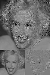 ☎∈ A hybrid image constructed from low-frequency components of a photograph of Marilyn Monroe (left inset) and high-frequency components of a photograph of Albert Einstein (right inset). The Einstein image is clearer in the full image.
 -

-
-

-

-
-
 ☎∈ A squircle (blue) compared with a rounded square (red). A squircle is a mathematical curve defined by the equation x4+y4=r4, while a rounded square is four 90° circular arcs of the same radius connected by tangent straight lines. In this construction, the two curves are arranged to coincide at angles which are multiples of 45° (i.e. 0°, 45°, 90°, 135° etc.).

.svg)

.svg)


Assorted photographs edit
United Kingdom edit
-
-
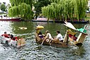 ☎∈ Some participants of the cardboard boat race on Suicide Sunday 2011 at the University of Cambridge.
 -
-

-

-

-
-

-
-

-
-
-

-
-
-

-

-

-

-
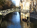 ☎∈ In the Mathematical Bridge, the straight lines (tangent to the bridge surface) lie outside the curved bridge surface.
 -
-
-
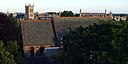 ☎∈ Cambridge skyline viewed from the Castle Mound. The roof in the foreground is part of St Giles church, the tower on the left is part of St John's College chapel, and the long tall building on the right is King's College Chapel.
 -

-
-
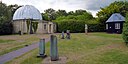
![☎∈ The 36-inch telescope at the Institute of Astronomy of the University of Cambridge being used for the 2011 Cambridge Astronomy Association Introduction to Astronomy course.[10]](//upload.wikimedia.org/wikipedia/commons/thumb/9/93/Cambridge_University_Institute_of_Astronomy_36_in_telescope.jpg/128px-Cambridge_University_Institute_of_Astronomy_36_in_telescope.jpg)
-
-
-

-

-
-
-

-

-

-

-
-
-
-
-

-

-

-
-

-

-
-
-
-
-
-

-
-
-
-

-

-

-
-

-

-

-

-
-

-

-

-
-

-

-
-
-

-
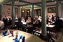
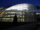
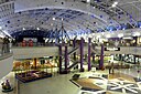
 ☎∈ High dynamic range view from the Leeds Corn Exchange balcony, of the west end of the interior in November 2010
 -
-
-
![☎∈ The Last Supper by Franz de Cleyn in the West Gallery of Windsor parish church of St John The Baptist. [11]](//upload.wikimedia.org/wikipedia/commons/thumb/9/9c/Windsor_parish_church_Last_Supper.jpg/128px-Windsor_parish_church_Last_Supper.jpg)
-
-
-

-
-
-

-

-
 ☎∈ The Regency TR-1 which used Texas Instruments' NPN transistors was the world's first commercially-produced transistor radio.
 -
-

-

-
-
-


.jpg)

.jpg)

.jpg)


![☎∈ The 36-inch telescope at the Institute of Astronomy of the University of Cambridge being used for the 2011 Cambridge Astronomy Association Introduction to Astronomy course.[10]](/wiki/File:Cambridge_University_Institute_of_Astronomy_36_in_telescope.jpg)


![☎∈ The Last Supper by Franz de Cleyn in the West Gallery of Windsor parish church of St John The Baptist. [11]](/wiki/File:Windsor_parish_church_Last_Supper.jpg)


Continental Europe edit


Taiwan edit


Singapore edit


Malaysia edit
-

-
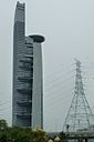
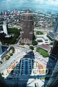 ☎∈ View to the northwest from the Petronas Towers skybridge, including the shadow of Tower 1 and the skybridge, and the Public Bank building.
 -

-

-

-

-

-
-
-
-
-

-

-

-
-
-

-

-
-
-
-
-
-
-
-
-

-

-

-


EasyTimeline edit
Template:Distance_from_Sun_using_EasyTimeline edit
☎ ∈ The following chart shows the range of distances of the planets, dwarf planets and Halley's Comet from the Sun.

Template:Hyperfocal_distance_depth_of_field_using_EasyTimeline edit
 Depths of field of 3 ideal lenses of focal lengths, f1, f2 and f3, and f-numbers N1, N2 and N3 when focused at objects at different distances. H1, H2 and H3 denote their respective hyperfocal distances (using Definition 1 in that article) with a circle of confusion of 0.03 mm diameter. The darker bars show how that, for fixed subject distance, the depth of field is increased by using a shorter focal length or smaller aperture. The second topmost bar of each set illustrates the configuration for a fixed focus camera with the focus permanently set at the hyperfocal distance to maximise the depth of field. |
Template:Tallest_building_history_using_EasyTimeline edit
☎ ∈ Timeline of recent buildings that have held the title Tallest building in the world. Heights of buildings are to scale. Note the early buildings that lost the title as their spires collapsed.

HTML edit
Chaffing and winnowing edit
| secure channel | insecure channel | |||||||||||||||||||||||||||||||||||||||||||||
| Alice | Charles | Bob | ||||||||||||||||||||||||||||||||||||||||||||
|---|---|---|---|---|---|---|---|---|---|---|---|---|---|---|---|---|---|---|---|---|---|---|---|---|---|---|---|---|---|---|---|---|---|---|---|---|---|---|---|---|---|---|---|---|---|---|
| constructs 4 packets, each containing one bit of her message and a valid MAC |
|
adds 4 chaff packets with inverted bits and invalid MAC, shown in italics (chaffing) |
|
discards packets with invalid MAC to recover the message (winnowing) | ||||||||||||||||||||||||||||||||||||||||||
In this example, Alice wishes to send the message "1001" to Bob. For simplicity, assume that all even MAC are valid and odd ones are invalid. | ||||||||||||||||||||||||||||||||||||||||||||||
Template:DiagnosticTesting Diagram edit
| Condition (as determined by "Gold standard") | ||||
| Condition Positive | Condition Negative | |||
| Test Outcome |
Test Outcome Positive |
True Positive | False Positive (Type I error) |
Positive predictive value = Σ True Positive Σ Test Outcome Positive
|
| Test Outcome Negative |
False Negative (Type II error) |
True Negative | Negative predictive value = Σ True Negative Σ Test Outcome Negative
| |
| Sensitivity = Σ True Positive Σ Condition Positive
|
Specificity = Σ True Negative Σ Condition Negative
| |||
2011_E._coli_O104:H4_outbreak edit

| LEGEND | No food restrictions | Food sale/trade restrictions / ran tests |
|---|---|---|
| No cases | ||
| Suspected cases | ||
| Known cases | ||
| Deaths |
| Country | Deaths | Confirmed cases | Suspected cases |
|---|---|---|---|
| 17[14] | 450 | 1 200 | |
| 0 | 3 | - | |
| 1 | 41 | - | |
| 0 | 14 | 26 | |
| 0 | 2 | - | |
| 0 | 0 | 3[15] | |
| 0 | 1[16] | - | |
| 0 | - | - | |
| 0 | - | - | |
| 0 | 2 | - | |
| 0 | - | 1 | |
| 0 | 1 | - | |
| 0 | 3 | - |
Uniform circular motion edit
|v| r
|
1 m/s 3.6 km/h 2.2 mph |
2 m/s 7.2 km/h 4.5 mph |
5 m/s 18 km/h 11 mph |
10 m/s 36 km/h 22 mph |
20 m/s 72 km/h 45 mph |
50 m/s 180 km/h 110 mph |
100 m/s 360 km/h 220 mph | |
|---|---|---|---|---|---|---|---|---|
| Slow walk | Bicycle | City car | Aerobatics | |||||
| 10 cm 3.9 in |
Laboratory centrifuge |
10 m/s² 1.0 g |
40 m/s² 4.1 g |
250 m/s² 25 g |
1.0 km/s² 100 g |
4.0 km/s² 410 g |
25 km/s² 2500 g |
100 km/s² 10000 g |
| 20 cm 7.9 in |
5.0 m/s² 0.51 g |
20 m/s² 2.0 g |
130 m/s² 13 g |
500 m/s² 51 g |
2.0 km/s² 200 g |
13 km/s² 1300 g |
50 km/s² 5100 g | |
| 50 cm 1.6 ft |
2.0 m/s² 0.20 g |
8.0 m/s² 0.82 g |
50 m/s² 5.1 g |
200 m/s² 20 g |
800 m/s² 82 g |
5.0 km/s² 510 g |
20 km/s² 2000 g | |
| 1 m 3.3 ft |
Playground carousel |
1.0 m/s² 0.10 g |
4.0 m/s² 0.41 g |
25 m/s² 2.5 g |
100 m/s² 10 g |
400 m/s² 41 g |
2.5 km/s² 250 g |
10 km/s² 1000 g |
| 2 m 6.6 ft |
500 mm/s² 0.051 g |
2.0 m/s² 0.20 g |
13 m/s² 1.3 g |
50 m/s² 5.1 g |
200 m/s² 20 g |
1.3 km/s² 130 g |
5.0 km/s² 510 g | |
| 5 m 16 ft |
200 mm/s² 0.020 g |
800 mm/s² 0.082 g |
5.0 m/s² 0.51 g |
20 m/s² 2.0 g |
80 m/s² 8.2 g |
500 m/s² 51 g |
2.0 km/s² 200 g | |
| 10 m 33 ft |
Roller-coaster vertical loop |
100 mm/s² 0.010 g |
400 mm/s² 0.041 g |
2.5 m/s² 0.25 g |
10 m/s² 1.0 g |
40 m/s² 4.1 g |
250 m/s² 25 g |
1.0 km/s² 100 g |
| 20 m 66 ft |
50 mm/s² 0.0051 g |
200 mm/s² 0.020 g |
1.3 m/s² 0.13 g |
5.0 m/s² 0.51 g |
20 m/s² 2 g |
130 m/s² 13 g |
500 m/s² 51 g | |
| 50 m 160 ft |
20 mm/s² 0.0020 g |
80 mm/s² 0.0082 g |
500 mm/s² 0.051 g |
2.0 m/s² 0.20 g |
8.0 m/s² 0.82 g |
50 m/s² 5.1 g |
200 m/s² 20 g | |
| 100 m 330 ft |
Freeway on-ramp |
10 mm/s² 0.0010 g |
40 mm/s² 0.0041 g |
250 mm/s² 0.025 g |
1.0 m/s² 0.10 g |
4.0 m/s² 0.41 g |
25 m/s² 2.5 g |
100 m/s² 10 g |
| 200 m 660 ft |
5.0 mm/s² 0.00051 g |
20 mm/s² 0.0020 g |
130 m/s² 0.013 g |
500 mm/s² 0.051 g |
2.0 m/s² 0.20 g |
13 m/s² 1.3 g |
50 m/s² 5.1 g | |
| 500 m 1600 ft |
2.0 mm/s² 0.00020 g |
8.0 mm/s² 0.00082 g |
50 mm/s² 0.0051 g |
200 mm/s² 0.020 g |
800 mm/s² 0.082 g |
5.0 m/s² 0.51 g |
20 m/s² 2.0 g | |
| 1 km 3300 ft |
High-speed railway |
1.0 mm/s² 0.00010 g |
4.0 mm/s² 0.00041 g |
25 mm/s² 0.0025 g |
100 mm/s² 0.010 g |
400 mm/s² 0.041 g |
2.5 m/s² 0.25 g |
10 m/s² 1.0 g |
I'm My Own Grandpa edit
| Narrator — Wife | |
| Father — Stepdaughter | |
| Narrator |
Family tree showing how
the narrator of the song
is his own grandfather.
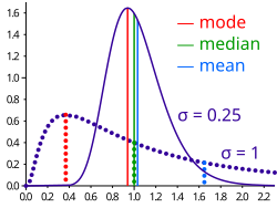
Mode (statistics) edit
When X has standard deviation σ = 0.25, the distribution of Y is weakly skewed. Using formulas for the log-normal distribution, we find:

Indeed, the median is about one third on the way from mean to mode.
When X has a larger standard deviation, σ = 1, the distribution of Y is strongly skewed. Now

Here, Pearson's rule of thumb fails.
Common logarithm edit
The following example uses the bar notation to calculate 0.012 × 0.85 = 0.0102:

* This step makes the mantissa between 0 and 1, so that its antilog (10mantissa) can be looked up.
Psychological pricing edit
| Ending | Percentage | |
|---|---|---|
| 0 | 7.5 | |
| 1 | 0.3 | |
| 2 | 0.3 | |
| 3 | 0.8 | |
| 4 | 0.3 | |
| 5 | 28.6 | |
| 6 | 0.3 | |
| 7 | 0.4 | |
| 8 | 1.0 | |
| 9 | 60.7 | |
Ratio of volumes of a cone, sphere and cylinder of the same radius and height edit

The above formulas can be used to show that the volumes of a cone, sphere and cylinder of the same radius and height are in the ratio 1 : 2 : 3, as follows.
Let the radius be r and the height be h (which is 2r for the sphere).

The discovery of the 2 : 3 ratio of the volumes of the sphere and cylinder is credited to Archimedes.[17]
Ratio of surface areas of a sphere and cylinder of the same radius and height edit
The above formulas can be used to show that the volumes of a sphere and cylinder of the same radius and height are in the ratio 2 : 3, as follows.
Let the radius be r and the height be h (which is 2r for the sphere).

.svg&action=edit&redlink=1)
.svg&action=edit&redlink=1)
.jpg&action=edit&redlink=1)
.jpg)
.jpg&action=edit&redlink=1)
.jpg)
.jpg&action=edit&redlink=1)
.jpg)
The discovery of this ratio is credited to Archimedes.[18]
Solar eclipse edit
| Moon | Sun | |||
|---|---|---|---|---|
| At perigee (nearest) |
At apogee (farthest) |
At perihelion (nearest) |
At aphelion (farthest) | |
| Mean radius, r | 1,737.10 kilometres (1,079.38 miles) |
696,000 kilometres (432,000 miles) | ||
| Distance, d | 363,104 km (225,622 mi) |
405,696 km (252,088 mi) |
147,098,070 km (91,402,500 mi) |
152,097,700 km (94,509,100 mi) |
| Angular diameter, 2×arctan(r / d) |
32' 54" (0.5482°) |
29' 26" (0.4907°) |
32' 32" (0.5422°) |
31' 28" (0.5244°) |
| Apparent size to scale |
 |
|
 |
|
| Rank in descending order |
1st | 4th | 2nd | 3rd |
Angular diameter edit
| Celestial body | Angular diameter | Relative size (10 pixels per arcsecond) |
|---|---|---|
| Sun | 31.6′ – 32.7′ | 28.7 – 29.7 times the maximum value for Venus (orange bar below) |
| Moon | 29.3′ – 34.1′ | 26.6 – 31.0 times the maximum value for Venus (orange bar below) |
| Venus | 9.565″ – 66.012″ | |
| Jupiter | 29.800″ – 50.115″ | |
| Saturn | 14.991″ – 20.790″ | |
| Mars | 3.492″ – 25.113″ | |
| Mercury | 4.535″ – 13.019″ | |
| Uranus | 3.340″ – 4.084″ | |
| Neptune | 2.179″ – 2.373″ | |
| Ceres | 0.330″ – 0.840″ | |
| Vesta | 0.20" – 0.64" | |
| Pluto | 0.063″ – 0.115″ | |
| R Doradus | 0.052″ – 0.062″ | |
| Betelgeuse | 0.049″ – 0.060″ | |
| Eris | 0.034" – 0.089″ | |
| Alphard | 0.00909″ | |
| Alpha Centauri A | 0.007″ | |
| Canopus | 0.006″ | |
| Sirius | 0.005936″ | |
| Altair | 0.003″ | |
| Deneb | 0.002″ | |
| Proxima Centauri | 0.001″ |
Apparent magnitude edit
| Visible to typical human eye |
Apparent magnitude |
Brightness relative to Vega |
Number of stars brighter than apparent magnitude[19] |
|---|---|---|---|
| Yes | -1 | 250% | 1 |
| 0 | 100% | 4 | |
| 1 | 40% | 15 | |
| 2 | 16% | 48 | |
| 3 | 6.3% | 171 | |
| 4 | 2.5% | 513 | |
| 5 | 1.0% | 1 602 | |
| 6 | 0.40% | 4 800 | |
| No | 7 | 0.16% | 14 000 |
| 8 | 0.063% | 42 000 | |
| 9 | 0.025% | 121 000 | |
| 10 | 0.010% | 340 000 |
Magnitude (astronomy) edit
| Apparent magnitude |
Brightness relative to magnitude 0 |
Example | Apparent magnitude |
Brightness relative to magnitude 0 |
Example | Apparent magnitude |
Brightness relative to magnitude 0 |
Example | ||
|---|---|---|---|---|---|---|---|---|---|---|
| -27 | 6.3×10¹⁰ | Sun | -7 | 630 | SN 1006 supernova | 13 | 6.3×10⁻⁶ | 3C 273 quasar | ||
| -26 | 2.5×10¹⁰ | -6 | 250 | International Space Station (max) | 14 | 2.5×10⁻⁶ | Pluto (max) | |||
| -25 | 1.0×10¹⁰ | -5 | 100 | Venus (max) | 15 | 1.0×10⁻⁶ | ||||
| -24 | 4.0×10⁹ | -4 | 40 | 16 | 4.0×10⁻⁷ | Charon (max) | ||||
| -23 | 1.6×10⁹ | -3 | 16 | Jupiter (max) | 17 | 1.6×10⁻⁷ | ||||
| -22 | 6.3×10⁸ | -2 | 6.3 | Mercury (max) | 18 | 6.3×10⁻⁸ | ||||
| -21 | 2.5×10⁸ | -1 | 2.5 | Sirius | 19 | 2.5×10⁻⁸ | ||||
| -20 | 1.0×10⁸ | 0 | 1.0 | Vega | 20 | 1.0×10⁻⁸ | ||||
| -19 | 4.0×10⁷ | 1 | 0.40 | Antares | 21 | 4.0×10⁻⁹ | Callirrhoe (small satellite of Jupiter) | |||
| -18 | 1.6×10⁷ | 2 | 0.16 | Polaris | 22 | 1.6×10⁻⁹ | ||||
| -17 | 6.3×10⁶ | 3 | 0.063 | Andromeda galaxy | 23 | 6.3×10⁻¹⁰ | ||||
| -16 | 2.5×10⁶ | 4 | 0.025 | Acubens | 24 | 2.5×10⁻¹⁰ | ||||
| -15 | 1.0×10⁶ | 5 | 0.010 | Vesta asteroid (max) | 25 | 1.0×10⁻¹⁰ | Fenrir (small satellite of Saturn) | |||
| -14 | 4.0×10⁵ | 6 | 4.0×10⁻³ | typical limit of naked eye | 26 | 4.0×10⁻¹¹ | ||||
| -13 | 1.6×10⁵ | Full moon | 7 | 1.6×10⁻³ | Ceres (max) | 27 | 1.6×10⁻¹¹ | visible light limit of 8m ground-based telescopes | ||
| -12 | 6.3×10⁴ | 8 | 6.3×10⁻⁴ | Neptune (max) | 28 | 6.3×10⁻¹² | ||||
| -11 | 2.5×10⁴ | 9 | 2.5×10⁻⁴ | 29 | 2.5×10⁻¹² | |||||
| -10 | 1.0×10⁴ | 10 | 1.0×10⁻⁴ | typical limit of 7x50 binoculars | 30 | 1.0×10⁻¹² | ||||
| -9 | 4.0×10³ | Iridium flare | 11 | 4.0×10⁻⁵ | 31 | 4.0×10⁻¹³ | ||||
| -8 | 1.6×10³ | 12 | 1.6×10⁻⁵ | 32 | 1.6×10⁻¹³ | visible light limit of Hubble Space Telescope |
Chroma subsampling edit
| 4:1:1 | 4:2:0 | 4:2:2 | 4:4:4 | ||||||||||||||||||||
| Y'CrCb | |||||||||||||||||||||||
| = | = | = | = | ||||||||||||||||||||
| Y' | |||||||||||||||||||||||
| + | + | + | + | ||||||||||||||||||||
| 1 | 2 | 3 | 4 | J = 4 | 1 | 2 | 3 | 4 | J = 4 | 1 | 2 | 3 | 4 | J = 4 | 1 | 2 | 3 | 4 | J = 4 | ||||
| (Cr, Cb) | 1 | a = 1 | 1 | 2 | a = 2 | 1 | 2 | a = 2 | 1 | 2 | 3 | 4 | a = 4 | ||||||||||
| 1 | b = 1 | b = 0 | 1 | 2 | b = 2 | 1 | 2 | 3 | 4 | b = 4 | |||||||||||||
| ¼ horizontal resolution, full vertical resolution |
½ horizontal resolution, ½ vertical resolution |
½ horizontal resolution, full vertical resolution |
full horizontal resolution, full vertical resolution |
||||||||||||||||||||
Template:DiagnosticTesting_Diagram edit
| This Wikipedia page has been superseded by template:diagnostic_testing_diagram and is retained primarily for historical reference. |
| True condition | |||||||
| Total population | Condition positive | Condition negative | Prevalence = Σ Condition positive/Σ Total population | Accuracy (ACC) = Σ True positive + Σ True negative/Σ Total population | |||
| Predicted condition positive |
True positive | False positive, Type I error |
Positive predictive value (PPV), Precision = Σ True positive/Σ Predicted condition positive | False discovery rate (FDR) = Σ False positive/Σ Predicted condition positive | |||
| Predicted condition negative |
False negative, Type II error |
True negative | False omission rate (FOR) = Σ False negative/Σ Predicted condition negative | Negative predictive value (NPV) = Σ True negative/Σ Predicted condition negative | |||
| True positive rate (TPR), Recall, Sensitivity (SEN), probability of detection, Power = Σ True positive/Σ Condition positive | False positive rate (FPR), Fall-out, probability of false alarm = Σ False positive/Σ Condition negative | Positive likelihood ratio (LR+) = TPR/FPR | Diagnostic odds ratio (DOR) = LR+/LR− | Matthews correlation coefficient (MCC) = √TPR·TNR·PPV·NPV − √FNR·FPR·FOR·FDR |
F1 score = 2 · PPV · TPR/PPV + TPR = 2 · Precision · Recall/Precision + Recall | ||
| False negative rate (FNR), Miss rate = Σ False negative/Σ Condition positive | Specificity (SPC), Selectivity, True negative rate (TNR) = Σ True negative/Σ Condition negative | Negative likelihood ratio (LR−) = FNR/TNR | |||||
Template:DiagnosticTesting_Example edit
| This Wikipedia page has been superseded by template:diagnostic_testing_example and is retained primarily for historical reference. |
| Patients with bowel cancer (as confirmed on endoscopy) | ||||||
| Total population (pop.) = 2030 |
Condition positive | Condition negative | Prevalence = (TP + FN) / pop.
= (20 + 10) / 2030 ≈ 1.48% |
Accuracy (ACC) = (TP + TN) / pop.
= (20 + 1820) / 2030 ≈ 90.64% | ||
| Fecal occult blood screen test outcome |
Test outcome positive |
True positive (TP) = 20 (2030 × 1.48% × 67%) |
False positive (FP) = 180 (2030 × (100% − 1.48%) × (100% − 91%)) |
Positive predictive value (PPV), precision = TP / (TP + FP)
= 20 / (20 + 180) = 10% |
False discovery rate (FDR) = FP / (TP + FP)
= 180 / (20 + 180) = 90.0% | |
| Test outcome negative |
False negative (FN) = 10 (2030 × 1.48% × (100% − 67%)) |
True negative (TN) = 1820 (2030 × (100% − 1.48%) × 91%) |
False omission rate (FOR) = FN / (FN + TN)
= 10 / (10 + 1820) ≈ 0.55% |
Negative predictive value (NPV) = TN / (FN + TN)
= 1820 / (10 + 1820) ≈ 99.45% | ||
| True positive rate (TPR), recall, sensitivity = TP / (TP + FN)
= 20 / (20 + 10) ≈ 66.7% |
False positive rate (FPR), fall-out, probability of false alarm = FP / (FP + TN)
= 180 / (180 + 1820) = 9.0% |
Positive likelihood ratio (LR+) = TPR/FPR
= (20 / 30) / (180 / 2000) ≈ 7.41 |
Diagnostic odds ratio (DOR) = LR+/LR−
≈ 20.2 |
F1 score = 2 × precision × recall/precision + recall
≈ 0.174 | ||
| False negative rate (FNR), miss rate = FN / (TP + FN)
= 10 / (20 + 10) ≈ 33.3% |
Specificity, selectivity, true negative rate (TNR) = TN / (FP + TN)
= 1820 / (180 + 1820) = 91% |
Negative likelihood ratio (LR−) = FNR/TNR
= (10 / 30) / (1820 / 2000) ≈ 0.366 | ||||
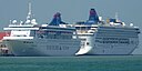
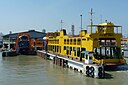
Penang Ferry Service edit
| Status | Configuration | Name | Year built | Deadweight tonnage | IMO ship identification number | Photograph |
|---|---|---|---|---|---|---|
| Retired | Passenger (upper deck) Vehicle (lower deck)[20] |
Pulau Labuan | 1971 | 139 | 7038408 | 
|
| In service | Passenger (upper deck) Vehicle (lower deck) |
Pulau Rawa | 1975 | 262 | 7343736 | 
|
| In service | Passenger (upper deck) Vehicle (lower deck) |
Pulau Talang Talang | 1975 | 262 | 7343748 | 
|
| In service | Passenger (upper deck) Vehicle (lower deck) |
Pulau Undan | 1975 | 262 | 7343724 | 
|
| In service | Vehicle (both decks) | Pulau Rimau | 1980 | 100 | 7911076 | 
|
| In service | Passenger (upper deck) Vehicle (lower deck) |
Pulau Angsa | 1981 | 100 | 8010491 | 
|
| In service | Vehicle (both decks) | Pulau Kapas | 1981 | 280 | 8101082 | 
|
| In service | Vehicle (both decks) | Pulau Payar | 2002 | 440 | 9254393 | 
|
| In service | Vehicle (both decks) | Pulau Pinang | 2002 | 440 | 9275244 | 
|
Day of Seven Billion edit
| Age group |
Estimated July 2010 population in millions[21] | |||||||||||
|---|---|---|---|---|---|---|---|---|---|---|---|---|
| Africa | Asia | Europe | Latin America and the Caribbean |
Northern America |
Oceania | |||||||
| 0–4 | 155.3 | 360.4 | 39.67 | 53.83 | 23.54 | 3.079 | ||||||
| 5–9 | 136.2 | 354.5 | 37.01 | 55.52 | 22.66 | 2.875 | ||||||
| 10–14 | 120.2 | 364.8 | 37.32 | 55.12 | 21.72 | 2.844 | ||||||
| 15–19 | 108.1 | 374.6 | 42.54 | 54.11 | 23.93 | 2.829 | ||||||
| 20–24 | 97.21 | 379.4 | 51.28 | 52.08 | 24.00 | 2.838 | ||||||
| 25–29 | 83.89 | 343.8 | 53.33 | 49.47 | 24.42 | 2.721 | ||||||
| 30–34 | 69.28 | 310.5 | 52.96 | 45.52 | 22.17 | 2.497 | ||||||
| 35–39 | 55.60 | 315.4 | 52.88 | 41.34 | 22.71 | 2.594 | ||||||
| 40–44 | 45.15 | 297.5 | 53.46 | 37.64 | 23.03 | 2.382 | ||||||
| 45–49 | 37.82 | 248.4 | 55.15 | 34.33 | 25.74 | 2.362 | ||||||
| 50–54 | 31.68 | 212.2 | 53.08 | 28.68 | 24.91 | 2.128 | ||||||
| 55–59 | 25.68 | 188.5 | 48.30 | 23.72 | 21.72 | 1.862 | ||||||
| 60–64 | 20.11 | 135.1 | 41.80 | 18.07 | 18.62 | 1.676 | ||||||
| 65–69 | 14.78 | 100.0 | 31.57 | 13.88 | 13.72 | 1.227 | ||||||
| 70–74 | 10.43 | 78.13 | 32.85 | 10.66 | 10.25 | 0.939 | ||||||
| 75–79 | 6.367 | 53.71 | 24.09 | 7.564 | 8.223 | 0.702 | ||||||
| 80–84 | 3.100 | 29.75 | 17.89 | 4.870 | 6.755 | 0.564 | ||||||
| 85–89 | 1.036 | 12.70 | 9.446 | 2.460 | 4.201 | 0.318 | ||||||
| 90–94 | 0.229 | 3.882 | 2.689 | 0.921 | 1.714 | 0.120 | ||||||
| 95–99 | 0.030 | 0.775 | 0.795 | 0.253 | 0.425 | 0.031 | ||||||
| 100+ | 0.003 | 0.090 | 0.089 | 0.044 | 0.063 | 0.004 | ||||||
Subpixel rendering edit
For example, consider an RGB Stripe Panel:
RGBRGBRGBRGBRGBRGB             WWWWWWWWWWWWWWWWWW         R = red
RGBRGBRGBRGBRGBRGB     is      WWWWWWWWWWWWWWWWWW         G = green
RGBRGBRGBRGBRGBRGB  perceived  WWWWWWWWWWWWWWWWWW  where  B = blue
RGBRGBRGBRGBRGBRGB     as      WWWWWWWWWWWWWWWWWW         W = white
RGBRGBRGBRGBRGBRGB             WWWWWWWWWWWWWWWWWW
Shown below is an example of black and white lines at the Nyquist limit, but at a slanting angle, taking advantage of Subpixel rendering to use a different phase each row:
RGB___RGB___RGB___             WWW___WWW___WWW___         R = red
_GBR___GBR___GBR__     is      _WWW___WWW___WWW__         G = green
__BRG___BRG___BRG_  perceived  __WWW___WWW___WWW_  where  B = blue
___RGB___RGB___RGB     as      ___WWW___WWW___WWW         _ = black
____GBR___GBR___GB             ____WWW___WWW___WW         W = white
Shown below is an example of chromatic aliasing when the traditional whole pixel Nyquist limit is exceeded:
RG__GB__BR__RG__GB             YY__CC__MM__YY__CC         R = red    Y = yellow
RG__GB__BR__RG__GB     is      YY__CC__MM__YY__CC         G = green  C = cyan
RG__GB__BR__RG__GB  perceived  YY__CC__MM__YY__CC  where  B = blue   M = magenta
RG__GB__BR__RG__GB     as      YY__CC__MM__YY__CC         _ = black
RG__GB__BR__RG__GB             YY__CC__MM__YY__CC
Circuit de Monaco edit
Article translation edit
References edit
- ^ Graham T. Smith (2002). Industrial metrology. Springer. p. 253. ISBN 1852335076.
{{cite book}}: Unknown parameter|isbn13=ignored (help) - ^ Geometric altitude vs. temperature, pressure, density, and the speed of sound derived from the 1962 U.S. Standard Atmosphere.
- ^ The World Bank - Life expectancy at birth, total (years)
- ^ World Population Prospects, the 2010 Revision
- ^ IMF World Economic Outlook database
- ^ Basics of space flight: Interplanetary Trajectories
- ^ "SINFONI in the Galactic Center: Young Stars and Infrared Flares in the Central Light-Month" by Eisenhauer et al, The Astrophysical Journal, 628:246-259, 2005
- ^ Galal Abada, "2004 On Site Review Report: Petronas Office Towers, Kuala Lumpur, Malaysia"
- ^ Note: The 2:1 pixel pattern in the near-isometric image allows smoother lines than in the isometric one.
- ^ Introduction to Astronomy – Week 4
- ^ The Parish Church of St. John The Baptist, Windsor. A History.
- ^ Case definition for HUS-cases associated with the outbreak in Germany
- ^ Noticia 20minutos.es
- ^ La OMS dice que la bacteria letal de Alemania pertenece a una cepa desconocida de 'E. coli'
- ^ Infected cucumbers: three suspicious cases in France . lemonde.fr. Retrieved on June 1st, 2011.
- ^ Hospitalizan a un hombre en San Sebastián por infección de 'E.coli'
- ^ Rorres, Chris. "Tomb of Archimedes: Sources". Courant Institute of Mathematical Sciences. Retrieved 2007-01-02.
- ^ Rorres, Chris. "Tomb of Archimedes: Sources". Courant Institute of Mathematical Sciences. Retrieved 2007-01-02.
- ^ "Magnitude". National Solar Observatory—Sacramento Peak. Archived from the original on 2008-02-06. Retrieved 2006-08-23.
- ^ "Off-limit zone held waiting folk: Captain", New Straits Times, 1 Mar 1989
- ^ File 1A: Total population (both sexes combined) by five-year age group, major area, region and country, annually for 1950-2010 (thousands)
^(?:Image|File):([^|]+)\|(?!\[\[File_talk:)
Image:$1|[[File_talk:$1|☎]][[Special:WhatLinksHere/$1|∈]]