Size of this preview: 800 × 568 pixels. Other resolutions: 320 × 227 pixels | 640 × 454 pixels | 1,024 × 726 pixels | 1,280 × 908 pixels.
Original file (1,280 × 908 pixels, file size: 55 KB, MIME type: image/png)
| This is a file from the Wikimedia Commons. Information from its description page there is shown below. Commons is a freely licensed media file repository. You can help. |
Summary
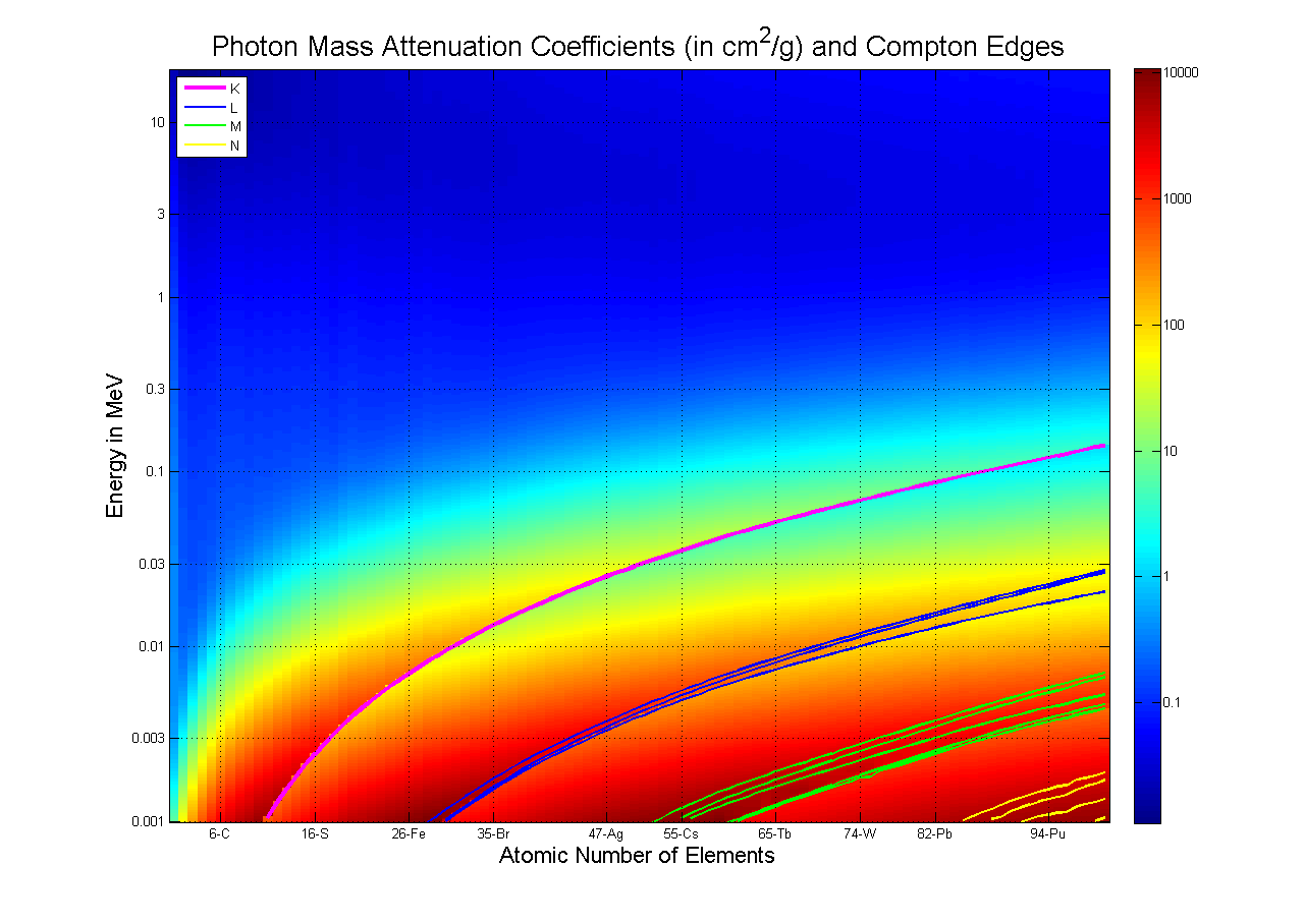
| Description | Photon Mass Attenuation Coefficient for photons in energy range from 1 keV to 20 MeV for Elements Z = 1 to 100. Based on [1]. Also shown are locations of Compton edges. |
| Date | |
| Source | Own work |
| Author | Jarekt |
| Other versions | SVG version of the same image can be found at Image:Photon Mass Attenuation Coefficients.svg, however it is larger and does not seem to render correctly |
This diagram was created with MATLAB.
The image was generated using the following MATLAB code, with help of external library PhotonAtenuattion2:
figure
Z = 1:100;  % elements with Z in 1-100 range - number of columns
nr = 500;   % number of rows to use in the plot
E = logspace(log10(0.001), log10(20), 500);  % define energy grid
[mac, CEdge] = PhotonAttenuationQ(Z, E);
colormap(jet(128)) % use hi-res color palette
imagesc(log10(mac));
grid on;
axis xy; % put small numbers on y axis on the bottom
title('Photon Mass Attenuation Coefficients (in cm^2/g) and Compton Edges');
xlabel('Atomic Number of Elements');
ylabel('Energy in MeV');
% Add X-Axis
EPos = [6 16 26 35 47 55 65 74 82 94];   % define array to store label location
ELab = { '6-C','16-S','26-Fe','35-Br','47-Ag','55-Cs','65-Tb','74-W','82-Pb','94-Pu'}; %Define Energy labels for y-axis
set(gca,'XTick'     ,EPos);
set(gca,'XTickLabel',ELab);
% Add Y-Axis
ELab = [0.001 0.003 0.01 0.03 0.1 0.3 1 3 10]; %Define Energy labels for y-axis
EPos = size(ELab);   % define array to store label location
for i=1:length(ELab), [tmp EPos(i)]=min(abs(E-ELab(i))); end
set(gca,'YTick'     ,EPos);
set(gca,'YTickLabel',ELab);
% add Colorbar
cbar_axes = colorbar;
set(cbar_axes,'YTick'     ,     -1:4 ); % The image is a log10 of the MAC ...
set(cbar_axes,'YTickLabel',10.^(-1:4)); % ... so add proper labels
hold on
% Add Conpton Edges to the plot
ed = accumarray([CEdge(:,1),CEdge(:,2)],CEdge(:,3)); % get per element energies of 14 compton edges
ed = 500*(log(ed')-log(0.001))/(log(20)-log(0.001)); % convert energy to row numbers of the image
K=plot(ed(:,1)    ,'m','LineWidth',3); %Plot K Compton edge
L=plot(ed(:, 2: 4),'b','LineWidth',2); %Plot 3 L Compton edges
M=plot(ed(:, 5: 9),'g','LineWidth',2); %Plot 5 M Compton edges
N=plot(ed(:,10:14),'Y','LineWidth',2); %Plot first 5 N Compton edges
legend([K(1),L(1),M(1),N(1)], {'K','L','M','N'}, 'Location', 'NorthWest');
Licensing
I, the copyright holder of this work, hereby publish it under the following licenses:

|
Permission is granted to copy, distribute and/or modify this document under the terms of the GNU Free Documentation License, Version 1.2 or any later version published by the Free Software Foundation; with no Invariant Sections, no Front-Cover Texts, and no Back-Cover Texts. A copy of the license is included in the section entitled GNU Free Documentation License. |
This file is licensed under the Creative Commons Attribution-Share Alike 3.0 Unported, 2.5 Generic, 2.0 Generic and 1.0 Generic license.
- You are free:
- to share – to copy, distribute and transmit the work
- to remix – to adapt the work
- Under the following conditions:
- attribution – You must give appropriate credit, provide a link to the license, and indicate if changes were made. You may do so in any reasonable manner, but not in any way that suggests the licensor endorses you or your use.
- share alike – If you remix, transform, or build upon the material, you must distribute your contributions under the same or compatible license as the original.
You may select the license of your choice.
File history
Click on a date/time to view the file as it appeared at that time.
| Date/Time | Thumbnail | Dimensions | User | Comment | |
|---|---|---|---|---|---|
| current | 01:36, 27 September 2007 | | 1,280 × 908 (55 KB) | Jarekt | {{Information |Description=Photon '''Mass Attenuation Coefficient''' for photons in energy range from 1 keV to 20 MeV for Elements Z = 1 to 100. Based on [http://physics.nist.gov/PhysRefData/XrayNoteB.html]. Also shown are locations of Compton edges. |Sou |
File usage
The following pages on the English Wikipedia use this file (pages on other projects are not listed):
Global file usage
The following other wikis use this file:
- Usage on ja.wikipedia.org