
Size of this PNG preview of this SVG file: 360 × 360 pixels. Other resolutions: 240 × 240 pixels | 480 × 480 pixels | 768 × 768 pixels | 1,024 × 1,024 pixels | 2,048 × 2,048 pixels.
Original file (SVG file, nominally 360 × 360 pixels, file size: 31 KB)
| This is a file from the Wikimedia Commons. Information from its description page there is shown below. Commons is a freely licensed media file repository. You can help. |
Summary
| Description |
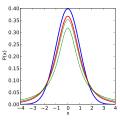
English: Student's t-distribution with 3 degrees of freedom. Enhanced plotting. |
| Date | |
| Source | Own work |
| Author | IkamusumeFan |
Plot using Python Matplotlib.
Licensing
I, the copyright holder of this work, hereby publish it under the following license:
This file is licensed under the Creative Commons Attribution-Share Alike 3.0 Unported license.
- You are free:
- to share – to copy, distribute and transmit the work
- to remix – to adapt the work
- Under the following conditions:
- attribution – You must give appropriate credit, provide a link to the license, and indicate if changes were made. You may do so in any reasonable manner, but not in any way that suggests the licensor endorses you or your use.
- share alike – If you remix, transform, or build upon the material, you must distribute your contributions under the same or compatible license as the original.
import numpy as np
import matplotlib.pyplot as plt
import scipy.special as sp

X = np.arange(-4, 4, 0.01)	# range of the graph

plt.clf()
plt.figure(figsize=(4,4))
plt.axes([0.17,0.13,0.79,0.8])
plt.hold(True)

Q = []	# No curves at first.

# Draw the curve of Normal distribution
mu = 0	# mean = 0
sigma = 1	# variance = 1
A = 1/(sigma*np.sqrt(2*np.pi))
B = np.exp(-(X-mu)*(X-mu)/(2*sigma*sigma));
Y = A*B
a = plt.plot(X, Y, '-', color='blue', lw=2)
Q.append(a)

# Draw the curve of Student's t-distribution
mu = 0	# mean = 0
nu = 3	# freedom degree = 3
A = np.exp(sp.gammaln((nu+1)/2.0));
B = np.exp(sp.gammaln(nu/2.0))*np.sqrt(nu*np.pi);
C = (1+X*X/nu)**(-(nu+1)/2.0);
Y = A*C/B;
a = plt.plot(X, Y, '-', color='red', lw=2)
Q.append(a)

# Draw the previous Student's t-distributions
for previous_nu in range(1,nu):
	mu = 0	# mean = 0
	A = np.exp(sp.gammaln((previous_nu+1)/2.0));
	B = np.exp(sp.gammaln(previous_nu/2.0))*np.sqrt(previous_nu*np.pi);
	C = (1+X*X/previous_nu)**(-(previous_nu+1)/2.0);
	Y = A*C/B;
	a = plt.plot(X, Y, '-', color='green', lw=1)
	Q.append(a)

# Remaining steps to finish drawing the graph.
plt.xlabel("x")
plt.ylabel("P(x)")
plt.xlim(-4,4)

# Saving the output.
plt.savefig("T_distribution_1df.pdf")
plt.savefig("T_distribution_1df.eps")
plt.savefig("T_distribution_1df.svg")
File history
Click on a date/time to view the file as it appeared at that time.
| Date/Time | Thumbnail | Dimensions | User | Comment | |
|---|---|---|---|---|---|
| current | 04:40, 21 July 2013 | | 360 × 360 (31 KB) | IkamusumeFan | The previous image is wrong on the degrees of freedom. |
| 03:56, 21 July 2013 |  | 360 × 360 (31 KB) | IkamusumeFan | User created page with UploadWizard |
File usage
The following pages on the English Wikipedia use this file (pages on other projects are not listed):
Global file usage
The following other wikis use this file:
- Usage on ca.wikipedia.org
- Usage on el.wikipedia.org
- Usage on ru.wikipedia.org
- Usage on sr.wikipedia.org
- Usage on zh.wikipedia.org