Constant314

Waveguides with certain symmetries may be solved using the method of separation of variables. Rectangular wave guides may be solved in rectangular coordinates.^[2]^: 143 Round waveguides may be solved in cylindracal coordinates.^[2]^: 198

[6]

Talk:Speed_of_electricity#Incorrect section: Speed of electromagnetic waves in good conductors

~~Some text with strike through.~~

Talk:Displacement current

Talk:Displacement current#Untrue assumptions in the “Current in capacitors” sub section

 ********************************************************************************

This topic should always be on the top.

*** some HTML ***

curl E = - $\partial$ B/ $\partial$ t

curl H = $\partial$ D/ $\partial$ t + J_conduction + J_source = curl H = $\partial$ D/ $\partial$ t + σE + J_source

where σ = conductivity

User:Constant314/Tow-Thomas active filter

\mathbf {E} =-\mathbf {\nabla } \phi -{\frac {\partial \mathbf {A} }{\partial t}},\,

Add alternate explanations of skin effect.

Add magnetic vector potential to the transformer page.

Telegrapher's equations edit

The solutions of the telegrapher's equations^[3]^{: 381–392} are functions of two parameters which are the propagation constant, $\gamma$ , and the characteristic impedance, $Z_{c}$ . The propagation constant is often written as $\gamma =\alpha +j\beta$ where $\alpha$ is called the attenuation constant and $\beta$ is called the phase constant. The natural units for $\alpha$ and $\beta$ are nepers per unit length and radians per unit length, respectively.

There are two solutions which can be interpreted as a forward propagating wave and a reverse propagating wave. The forward wave, which has a voltage of $V_{F}(x)$ and a current of $I_{F}(x)$ , is given by:

V_{F}(x)=V_{(F,0)}e^{-\gamma x}

I_{F}(x)={\frac {V_{F}(x)}{Z_{c}}}

The reverse wave, which has a voltage of $V_{R}(x)$ and a current of $I_{R}(x)$ , is given by:

V_{R}(x)=V_{(R,d)}e^{-\gamma (d-x)}

I_{R}(x)=-{\frac {V_{R}(x)}{Z_{c}}}

where

\gamma =\alpha +j\beta ={\sqrt {(R+j\omega L)(G+j\omega C)}}

.^[3]^: 385

Z_{c}={\sqrt {\frac {(R+j\omega L)}{(G+j\omega C)}}}

</math>.^[3]^: 385

v={\frac {\omega }{\beta }}

= the propagation velocity.

\lambda ={\frac {2\pi }{\beta }}

= wavelength.

d

= length of the transmission line.

V_{(F,0)}

= a constant that depends on conditions at

x=0

.

V_{(F,d)}

= a constant that depends on conditions at

x=d

.

The negative sign in the expression for $I_{R}(x)$ indicates that the current in the reverse wave is traveling in a direction that is opposite to the reference direction, which is the direction of the forward propagating wave. $Z_{c},\gamma ,\alpha ,\beta ,\lambda ,$ and $v$ are secondary parameters which means that they can be expressed in terms of the primary parameters $R,G,L,$ and $C$ .

The effect of inductive loading on the velocity of an underwater cable.

Regimes edit

The propagation constant and the characteristic impedance may be factored as

Z_{c}=Z_{0}{\sqrt {\frac {(1+r_{\omega })}{(1+g_{\omega })}}}

.

\gamma =j{\frac {\omega }{v_{0}}}{\sqrt {(1+r_{\omega })(1+g_{\omega })}}

.

where

Z_{0}={\sqrt {\frac {L}{C}}}

= nominal high frequency impedance.

v_{0}={\frac {1}{\sqrt {LC}}}

= nominal high frequency phase velocity.

r_{\omega }={\frac {R}{j\omega L}}

= impedance ratio.

g_{\omega }={\frac {G}{j\omega C}}

= admittance ratio.

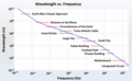
where The terms $v_{0}$ and $Z_{0}$ are relatively independent of frequency. The frequency dependent behavior of $\gamma$ and $Z_{c}$ can be separated into nine regions according to whether the ratios $g_{\omega }$ and $r_{\omega }$ are much less than unity, much greater than unity or about equal to unity. In practice, four of the combinations do not occur leaving five regions from DC to high frequency.

Ratio of G/ωC and R/ωL versus frequency for a typical RG-59 coaxial transmission line with a good (high resistivity) dielectric insulator.

Phase velocity of a typical RG-59 coaxial transmission line with a good (high resistivity) dielectric insulator relative to the speed of light in vacuum.

The graph to the left shows the frequency dependent variation of $g_{\omega }$ and $r_{\omega }$ of a transmission line with a good dielectric such as high density polyethylene. Separation of the spectrum into regions has been arbitrarily set at the frequencies at which one of the ratios is either 0.1 or 10.

The five regions may be easily seen in the adjacent graph of velocity versus frequency of a transmission line with a good dielectric such as polyethylene:

From lowest to highest frequency the regions are:

Near DC (NDC) where ${\frac {G}{j\omega C}}>>1$ and ${\frac {R}{j\omega L}}>>1$
Very low frequency (VLF) where ${\frac {G}{j\omega C}}\approx 1$ and ${\frac {R}{j\omega L}}>>1$
Low frequency (LF) where ${\frac {G}{j\omega C}}<<1$ and ${\frac {R}{j\omega L}}>>1$
Intermediate frequency (IF) where ${\frac {G}{j\omega C}}<<1$ and ${\frac {R}{j\omega L}}\approx 1$
High frequency (HF) where ${\frac {G}{j\omega C}}<<1$ and ${\frac {R}{j\omega L}}<<1$

High frequency regime edit

The high frequency regime is most associated with transmission line behavior. It includes Ethernet, most broadcasting, ordinary video, computer buses, the higher portions of the digital telephony spectrum ( HDSL, ADSL, VDSL).

Z_{c}={\sqrt {\frac {L}{C}}}{\sqrt {\frac {(1+{\frac {R}{j\omega L}})}{(1+{\frac {G}{j\omega C}})}}}\approx {\sqrt {\frac {L}{C}}}(1+{\frac {R}{2j\omega L}}-{\frac {G}{2j\omega C}})

\gamma =j\omega {\sqrt {LC}}{\sqrt {(1+{\frac {R}{j\omega L}})(1+{\frac {G}{j\omega C}})}}\approx j\omega {\sqrt {LC}}(1+{\frac {R}{2j\omega L}}+{\frac {G}{2j\omega C}})=j\omega {\sqrt {LC}}+{\frac {R}{2}}{\sqrt {\frac {C}{L}}}+{\frac {G}{2}}{\sqrt {\frac {L}{C}}}

\alpha ={\frac {R}{2}}{\sqrt {\frac {C}{L}}}+{\frac {G}{2}}{\sqrt {\frac {L}{C}}}

\beta =\omega {\sqrt {LC}}

v={\frac {\omega }{\beta }}={\frac {1}{\sqrt {LC}}}

Intermediate frequency regime edit

The intermediate frequency regime includes the lower portions of the digital telephony spectrum (ISDN, HDSL, ADSL, the upper frequencies of music,

Low frequency regime edit

The low frequency regime includes voice telephony, the lower frequencies of music,

Very low frequency regime edit

The very low frequency regime includes

Near DC regime edit

If $G\equiv 0$ then there is no near DC regime. This is the case if the dielectric is vacuum.

The near DC regime expressions approach their DC values as frequency approaches zero, except wavelength which approaches infinity.

Z_{c}={\sqrt {\frac {R}{G}}}{\sqrt {\frac {(1+{\frac {j\omega L}{R}})}{(1+{\frac {j\omega C}{G}})}}}\approx {\sqrt {\frac {R}{G}}}

.

\gamma ={\sqrt {RG}}{\sqrt {(1+{\frac {j\omega L}{R}})(1+{\frac {j\omega C}{G}})}}\approx {\sqrt {RG}}(1+{\frac {j\omega L}{2R}}+{\frac {j\omega C}{2G}})

.

\alpha ={\sqrt {RG}}

.

\beta ={\sqrt {RG}}({\frac {\omega L}{2R}}+{\frac {\omega C}{2G}})

. Typically

{\frac {\omega C}{2G}}>>{\frac {\omega L}{2R}}

so

\beta \approx {\frac {\omega C}{2}}{\sqrt {\frac {R}{G}}}

.

v={\frac {2}{C}}{\sqrt {\frac {G}{R}}}

.

The near DC regime expressions approach their DC values as frequency approaches zero, except wavelength which approaches infinity.

Z_{c,dc}={\sqrt {\frac {R_{dc}}{G_{dc}}}}

.

\alpha _{dc}={\sqrt {R_{dc}G_{dc}}}

.

\beta _{dc}=0

v_{dc}={\frac {2}{C_{dc}}}{\sqrt {\frac {G_{dc}}{R_{dc}}}}

.

The following gallery shows the frequency dependence of some of the other secondary parameters.

Wavelength of a typical RG-59 coaxial transmission line with a good (high resistivity) dielectric insulator in meters.
Loss of a typical RG-59 coaxial transmission line with a good (high resistivity) dielectric insulator in dB/meter.
Magnitude of the characteristic impedance of a typical RG-59 coaxial transmission line with a good (high resistivity) dielectric insulator in ohms.
Phase of the characteristic impedance of a typical RG-59 coaxial transmission line with a good (high resistivity) dielectric insulator in degrees.

Gallery Example edit

Simple TDR made from lab equipment
Simple TDR made from lab equipment
TDR trace of a transmission line with an open termination
TDR trace of a transmission line with a short circuit termination
TDR trace of a transmission line with a 1nF capacitor termination
TDR trace of a transmission line with an almost ideal termination
TDR trace of a transmission line terminated on an oscilloscope high impedance input. The blue trace is the pulse as seen at the far end. It is offset so that the baseline of each channel is visible
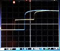TDR trace of a transmission line terminated on an oscilloscope high impedance input driven by a step input from a matched source. The blue trace is the signal as seen at the far end.

Phase velocity of a typical RG-59 coaxial transmission line with a good (high resistivity) dielectric insulator relative to the speed of light in vacuum.
Wavelength of a typical RG-59 coaxial transmission line with a good (high resistivity) dielectric insulator in meters.
Loss of a typical RG-59 coaxial transmission line with a good (high resistivity) dielectric insulator in dB/meter.
Magnitude of the characteristic impedance of a typical RG-59 coaxial transmission line with a good (high resistivity) dielectric insulator in ohms.
Phase of the characteristic impedance of a typical RG-59 coaxial transmission line with a good (high resistivity) dielectric insulator in degrees.

Ideal transformer has zero Magnetomotive force edit

This involves a slight bit of synthesis from Brenner and Javid. Page 599 gives i₂/i₁ = 1/n and 1/n = n₁/n₂ which can be combined by simple arithmetic to give i₁n₁ = i₂n₂ or i₁n₁ - i₂n₂ = 0.

Hayt & Kemmerly in Engineering Circuit Analysis, 5'th on page 446 state plainly that i₁n₁ = i₂n₂, but it doesn't seem worth adding a reference for that.

(i₁n₁ - i₂n₂) is the magnetomotive force, using the current reference directions given in the figure in the same section.

The role of the magnetic vector potential in transformers edit

First, an analogy. I can compute the velocity of my car by computing the time derivative of the number displayed on the odometer. That doesn’t mean the odometer causes the car’s velocity. The relationship holds because they are both caused by the same thing, which is the motor. Faraday's law of induction (FLI) states that the EMF (path integral of the electric field) in closed loop is proportional to the time derivative of the total flux the enclosed in the loop, including the flux in the core. This is a very useful relationship for designing transformers and predicting their behavior. This doesn’t mean that the flux in the core causes the EMF in the secondary, although it is often taught that way. Most of the time, that is good enough. But, in fact, if the flux in the core actually caused the EMF in the secondary, that would be action at a distance. Feynman makes this point in Volume 2 of the Feynman lectures, chap 15 section 5 in the second paragraph following equation 15.36.

Modern physicists have worked very hard to eliminate action at a distance. The modern formulation is that the currents produce the magnetic vector potential, A, at the wires. A produces a component of the electric field, E in accordance with E = -∂A/∂t (actually E= - $\nabla$ φ -∂A/∂t, but I am ignoring φ). The line integral of -∂A/∂t over a closed path is the EMF. Faraday’s law of induction (FLI) works because B = $\nabla \times$ A; E at the wires has the same cause as B in core. FLI is useful for engineers because they almost always have the transformer connected to a circuit which provides a complete path. However, E = -∂A/∂t, gives the E field at each infinitesimal part of the path.

I am not going to try to put this in the article; it is probably too technical. I’m going for WP:RIGHTGREATWRONGS, but I will try to edit the article so it is not in conflict with the modern formulation. For example, instead of “EMF is caused by the changing flux in the core” I may write “EMF is equal the rate of change of the flux in the core.” The first version is simpler and more direct, but it is a fiction whereas the second version is a correct statement.

Your comments are invited.

Apparently they knew this in 1913

https://books.google.com/books?id=71w2AQAAMAAJ&pg=PA947&lpg=PA947&dq=vector+potential+transformers&source=bl&ots=Sf4P9Qk63c&sig=n3sg0l_dPQ96fwIJT3tm-tzjF7g&hl=en&sa=X&ved=2ahUKEwjh9PGrgpLfAhWvna0KHTMNBrM4FBDoATAHegQIAxAB#v=onepage&q=vector%20potential%20transformers&f=false

And 1971

https://books.google.com/books?id=60EbAQAAMAAJ&pg=PA1195&dq=%22vector+potential%22+transformers&hl=en&sa=X&ved=0ahUKEwjk7KeAhJLfAhVKQ6wKHUKyDKAQ6AEIXzAJ#v=onepage&q=%22vector%20potential%22%20transformers&f=false

E-I core transformer edit

Magnetic flux path around the air gap in a transformer core made from E and I laminations. A:air gap. B: magnetic flux (blue dashed lines). E: E lamination. I: I lamination. G: Effective gap. S: surface treatment of laminations (gray). W: Windings.

Side view of transformer showing interleaved E-I laminations

Interleaved E-I transformer laminations showing air gap and flux paths

Some Picture Files edit

Files uploaded by Roy McCammon

A schematic representation of long distance electric power transmission. C=consumers, D=step down transformer, G=generator, I=current in the wires, Pe=power reaching the end of the transmission line, Pt=power entering the transmission line, Pw=power lost in the transmission line, R=total resistance in the wires, V=voltage at the beginning of the transmission line, U=step up transformer.

Depiction of a Gaussian pulse and related fields in a two-wire transmission line. The conductors are indicated by light orange. Green indicates the surface charge density with polarity signs in white. Red indicates surface current density with white direction arrows. Blue-gray indicates electric field intensity with blue direction arrow. Length of dashed brown arrows indicates displacement current density. Black arrows indicate direction of propagation.

AWG Formulae edit

By definition, the diameter of #. 36 AWG is 0.005 inches, and # 0000 is 0.46 inches. The ratio of these diameters is 1:92, and there are 40 gauge sizes from #. 36 to # 0000, or 39 steps. The diameter of a # n AWG wire is determined, for gauges smaller than # 00 (36 to 0), according to the following formula:

d_{n}=0.005~\mathrm {inch} \times 92^{\frac {36-n}{39}}=0.127~\mathrm {mm} \times 92^{\frac {36-n}{39}}

The gauge can be calculated from the diameter using

n=-39\log _{92}\left({\frac {d_{n}}{0.005~\mathrm {inch} }}\right)+36

n={\frac {-39}{\log _{10}92}}\log _{10}\left({\frac {d_{n}}{0.005~\mathrm {inch} }}\right)+36

n={\frac {-39}{\log _{e}92}}\log _{e}\left({\frac {d_{n}}{0.005~\mathrm {inch} }}\right)+36

Tansformer talk edit

In the ideal transformer section it notes that the ideal transformer is lossless, therefore power out = power in. If output volts go down then output current must go up. That’s a conclusion and not an explanation. Unfortunately, the reliable sources tend to write a bunch of equations and conclude that current transforms inversely with the turns ratio. Again it is a conclusion and not an explanation. I have an explanation, but without any reliable sources, it would be WP:OP. I’ll outline it here, hoping that maybe someone else can find a reliable source or determine that it is supportable by the sources already in the article. The gist is this, take a transformer with turns N_P and N_S and a load on the secondary and try to force a current I_P into the primary. If the quantity N_P × I_P – N_S × I_S ≠ 0, then you are forcing flux into the nominally infinite (or very large) self-inductance. It responds with an infinite (or very large) voltage seen on both the primary and the secondary. But there is a load on the secondary that would draw an infinite (or very large) current, so you can’t really get an infinite voltage. In fact, the secondary voltage that you can get is just enough to satisfy N_P × I_P – N_S × I_S = 0. The transformer, in effect, generates the voltage required to get the secondary current that will satisfy N_P × I_P – N_S × I_S = 0. A transformer with an infinite self-inductance is, so to speak, intolerant of N_P × I_P – N_S × I_S ≠ 0. You can sort of make a Lenz's law argument that any deviation from N_P × I_P – N_S × I_S = 0 would create huge reaction that would oppose the deviation.

Sounds about right. I might have done it in terms of Ampere-Turns, as are commonly used in magnet design problems. Gah4 (talk) 06:19, 22 September 2016 (UTC)

Velocity of electromagnetic waves edit

The speed of electromagnetic waves in a low-loss dielectric is given by

\quad v={\frac {1}{\sqrt {\epsilon \mu }}}={\frac {c}{\sqrt {\epsilon _{r}\mu _{r}}}}

.^[4]^: 346

where

\quad c

= speed of light in vacuum.

\quad \mu _{0}

= the permeability of free space = 4π x 10⁻⁷ H/m.

\quad \mu _{r}

= relative magnetic permeability of the material. Usually in good dielectrics,

\mu _{r}=1

.

\quad \mu

=

\mu _{r}

\mu _{0}

.

\quad \epsilon _{0}

= the permeability of free space.

\quad \epsilon _{r}

= relative magnetic permeability of the material. Usually in good conductors,

\epsilon _{r}=1

.

\quad \epsilon

=

\mu _{r}

\mu _{0}

.

The speed of electromagnetic waves in a good conductor is given by

\quad v={\sqrt {\frac {2\omega }{\sigma \mu }}}={\sqrt {\frac {4\pi }{\sigma _{c}\mu _{0}}}}{\sqrt {\frac {f}{\sigma _{r}\mu _{r}}}}\approx \left(0.41{\frac {\mathsf {m}}{\mathsf {s}}}\right){\sqrt {\frac {f}{\sigma _{r}\mu _{r}}}}

.^[4]^: 360

where

\quad f

= frequency.

\quad \omega

= angular frequency = 2πf.

\quad \sigma _{c}

= conductivity of annealed copper = 5.96 x 10⁷ S/m.

\quad \sigma _{r}

= conductivity of the material relative to the conductivity of copper. For hard drawn copper

\sigma _{r}

may be as low as 0.97.

\quad \sigma

=

\sigma _{r}\sigma _{c}

.

In copper at 60 Hz, $v\approx 3.2m/s$ . Some sprinters can run twice as fast. As a consequence of Snell's Law and the extremely low speed, electromagnetic waves always enter good conductors in a direction that is normal to the surface, regardless of the angle of incidence. This velocity is then the speed with which electromagnetic waves penetrate into the conductor and is not the Drift velocity of the conduction electrons.

Velocity in metal edit

I have seven reliable sources of which two use plain language and the others simple formulas to state that the speed of an electromagnetic wave propagating in a good conductor is very much slower than the speed of light.

Plain language

Hayt, (professor of electrical engineering emeritus at Purdue U.) ^[4]^: 346, Engineering Electromagnetics, 5th, McGraw-Hill,1989 page 360 states "...velocity and wavelength within a good conductor ... For copper at 60 Hz, λ=5.36 cm and v= 3.22 m/s, ..."

Kraus,(professor of electrical engineering and astronomy emeritus at Ohio State U.) Electromagnetics, page 451, Table 10-6 for copper gives velocity at 60Hz of 3.2 m/s

Simple formula^[5]^: 142

Balanis,(professor of electrical engineering at Arizona State U.) Advanced Engineering Electromagnetics, 2 ed, 2012, Wiley, page 142, TABLE 4-1 gives the velocity in a good conductor as

v\approx {\sqrt {{2\omega } \over {\mu \sigma }}}

Rao^[6]^: 332,(professor of electrical and computer engineering at U. of Illinois at Urbana) Elements of Engineering Electromagnetics page 332 equation 6.81c

v\approx {\sqrt {{4\pi f} \over {\mu \sigma }}}

Kraus, Electromagnetics, page 450, equation 11

v_{c}={\sqrt {{2\omega } \over {\sigma \mu }}}

Sadiku, Elements of Electromagnetics, 1989, p446, section 10.6 Plane waves in good conductors. equation (10.51)b

u={\sqrt {{2\omega } \over {\mu \sigma }}}

Taking

\omega =377

\mu =4\pi \times 10^{-7}

\sigma =5.96\times 10^{7}

yields

v\approx 3.17m/s

Two simple formulas^[7]^: 50–52

Harrington,(professor of electrical engineering at Syracuse U.) Time-Harmonic Electromagnetic Fields, 1961, McGraw-Hill, page 52 gives

v={{\omega } \over {k^{\prime }}}

and on page 50 gives for a good conductor

k^{\prime }={\sqrt {{\omega \mu \sigma } \over {2}}}

Using the previous values gives

k^{\prime }=118.81

v={377 \over 118.81}=3.17m/s

Stratton,(professor of physics emeritus at MIT) Electromagnetic Theory, 1941, McGraw-Hill, page 522

gives the wavelength within a conductor as

\lambda =2\pi {\sqrt {{2} \over {\omega \mu \sigma }}}

and by common knowledge

v=f\lambda ={\omega  \over {2\pi }}\lambda

yielding

v={\omega  \over {2\pi }}2\pi {\sqrt {{2} \over {\omega \mu \sigma }}}={\sqrt {{2\omega } \over {\mu \sigma }}}

Note that Jackson cites Stratton, Harrington, Sadiku, and Kraus

Jackson 2nd page 337 and 3'rd page 354, eq. 8.9 and 8.10 give the phase term for a wave propagating into the conductor as ${i\xi } \over \delta$ where ξ=depth into conductor and δ=skin depth.

Magnetic current edit

Magnetic current is, nominally, a fictitious current composed of fictitious moving magnetic mono-poles. It has the dimensions of volts. Magnetic currents produce an electric field analogously to the production of a magnetic field by electric currents. Magnetic current density is usually represented by the symbol M, which has the units of v/m² (volts per square meter). A given distibution of electric change can be mathematically replaced by an equivalent distribution of magnetic current. This fact can be used to simplify some electromagnetic field problems. ^[a] ^[b]

Magnetic current (flowing magnetic mono-poles), M, creates an electric field, E, in accordance with the left-hand rule.

The direction of the electric field produced by magnetic currents is determined by the left-hand rule (opposite to the right-hand rule) as evidenced by the negative sign in the equation curl E = -M. One component of M is the familiar term $\partial$ B/ $\partial$ t, which is referred to as the magnetic displacement current or more properly as the magnetic displacement current density. ^[c] ^[d] ^[e]

^[10]

^[11]^: 286

^[f]^: 291

^[g]^: 291

Galilean electromagnetism edit

$E'=E+{\frac {v}{c}}\times B$

$B'=B-{\frac {v}{c}}\times E$

$H'=H-v\times D$

As late as 1963, Purcell offered the following low velocity transformations as suitable for calculating the electric field experienced by a jet plane tranvelling in the Earth's magnetic field.

E'=E+v\times B

.

B'=B-\epsilon _{0}\mu _{0}v\times E

. ^[h]^: 222

In 1973 Bellac and Levy-Leblond state that these equations are incorrect or misleading because they do not correspond to any consistent Galilean limit. Rousseaux gives a simple example showing that a transformation from an initial inertial frame to a second frame with a speed of v₀ with respect to the first frame and then to a third frame moving with a speed v₁ with respect to the second frame would give a result different from going directly from the first frame to the third frame using a relative speed of (v₀ + v₁).

Bellac and Levy-Leblond offer two transformations that do have consistent Galilean limits as follows:

The electric limit applies when electric field effects are dominant such as when Faraday's law of induction was insignificant.

E'=E

.

B'=B-\epsilon _{0}\mu _{0}v\times E

.

The magnetic limit applies when the magnetic field effects are dominant.

E'=E+v\times B

.

B'=B

.

Statement by Germain Rousseaux: "For the experiments of electrodynamics of moving bodies with low speeds, the Galilean theory is the most adapted because it is easier of stake in work from the calculus point of view and does not bring in the kinematics effect of Special Relativity which are absolutely unimportant in the Galilean limit.^[13]^: 12.

Volt, voltage, EMF and Potential edit

My 2 cents worth.

Volt is about the unit of measurement and should be a separate article.

Everything else is tied together by the equation E = -∇(φ) -σA/σt, where φ is the electrodynamic retarded electric scalar potential and A is the retarded magnetic vector potential.

Voltage is, to me, a circuit quantity. It’s what a voltmeter would read between two points in a circuit. If the leads to the voltmeter went through a region where σA/σt ≠ 0, then the voltmeter reading would depend on the path of the leads to the voltmeter and the voltage would be ill defined.

Electromotive force, I usually associate with a path integral of the electric field (as defined above) tangential to a definite path. Usually the path follows a conductor. Typical paths may include a battery, generator, transformer, loop antenna, microphone, transducer. EMF for a specific path is unique. The path may be implicit. In a particular usage, there may be no mention of the path integral, but it is there never-the-less. If the beginning point and ending point of the path integral were in a continuous region where σA/σt = 0 then the voltage measured between those points by a voltmeter connected to those points and entirely in the region would read a unique value and EMF would numerically be the same as the voltage.

Potential has more than one meaning. The article will have to deal with that. For me, potential is a field quantity, although potential is used as a synonym for voltage in both DC and AC circuits.

- The electrodynamic retarded scalar electric potential, which is used above in the equation for E. It is well defined everywhere except for points occupied by point charges. The difference in potential between two points is also well defined but may be physically meaningless. In general, the potential difference between two points is not the voltage between those two points.

- The electrostatic potential that applies to electrostatics and DC circuits or any situation where σA/σt = 0. In this case, the difference in potential between two points is the same as the voltage between those two points and EMF evaluated along any path is also equal to the same voltage.^[14] ^[15] ^[16] ^[17]

If you use a definition of circuit like a roughly circular line, route, or movement that starts and finishes at the same place. That is, a mathematical definition, then path and circuit are similar. But in EE, circuit has a different definition. Gah4 (talk) 06:28, 22 September 2016 (UTC)

Good morning Gah4. Thanks for your comments. I use my user page to prepare comments to be pasted into other pages, so they may not make any sense unless seen in the context of the target page. Also, I may edit them on the target page, but I don't come back here an echo the edits. So, what you find here may be incorrect, incomplete or obsolete and I don't make any attempt to maintain it. In this particular case, circuit means whatever it means in the target article, which was probably Faraday's law of induction. Comments and suggestions are welcome on that article's talk page. Cheers. Constant314 (talk) 14:27, 22 September 2016 (UTC)

That is what I suspected. Your talk page is on my watch list from a previous discussion, and so I happened to see it. The one on wire gauge is interesting. I never saw the formula listed before, and didn't even know that there was one. I wasn't looking in too much detail, though. Sometimes I am not ready for a real talk page discussion. Thanks, Gah4 (talk) 14:48, 22 September 2016 (UTC)

Quantities and units edit

_________________________________________________________

Electromagnetic units are part of a system of electrical units based primarily upon the magnetic properties of electric currents, the fundamental SI unit being the ampere. The units are:

ampere (electric current)
coulomb (electric charge)
farad (capacitance)
henry (inductance)
ohm (resistance)
tesla (magnetic flux density)
volt (electric potential)
watt (power)
weber (magnetic flux)

In the electromagnetic cgs system, electric current is a fundamental quantity defined via Ampère's law and takes the permeability as a dimensionless quantity (relative permeability) whose value in a vacuum is unity. As a consequence, the square of the speed of light appears explicitly in some of the equations interrelating quantities in this system.

SI electromagnetism units v t e
Symbol^[18]	Name of Quantity	Derived Units	Unit	Base Units
I	electric current	ampere (SI base unit)	A	A (= W/V = C/s)
Q	electric charge	coulomb	C	A⋅s
U, ΔV, Δφ; E	potential difference; electromotive force	volt	V	kg⋅m²⋅s⁻³⋅A⁻¹ (= J/C)
R; Z; X	electric resistance; impedance; reactance	ohm	Ω	kg⋅m²⋅s⁻³⋅A⁻² (= V/A)
ρ	resistivity	ohm metre	Ω⋅m	kg⋅m³⋅s⁻³⋅A⁻²
P	electric power	watt	W	kg⋅m²⋅s⁻³ (= V⋅A)
C	capacitance	farad	F	kg⁻¹⋅m⁻²⋅s⁴⋅A² (= C/V)
E	electric field strength	volt per metre	V/m	kg⋅m⋅s⁻³⋅A⁻¹ (= N/C)
D	electric displacement field	coulomb per square metre	C/m²	A⋅s⋅m⁻²
ε	permittivity	farad per metre	F/m	kg⁻¹⋅m⁻³⋅s⁴⋅A²
χ_e	electric susceptibility	(dimensionless)	–	–
G; Y; B	conductance; admittance; susceptance	siemens	S	kg⁻¹⋅m⁻²⋅s³⋅A² (= Ω⁻¹)
κ, γ, σ	conductivity	siemens per metre	S/m	kg⁻¹⋅m⁻³⋅s³⋅A²
B	magnetic flux density, magnetic induction	tesla	T	kg⋅s⁻²⋅A⁻¹ (= Wb/m² = N⋅A⁻¹⋅m⁻¹)
Φ	magnetic flux	weber	Wb	kg⋅m²⋅s⁻²⋅A⁻¹ (= V⋅s)
H	magnetic field strength	ampere per metre	A/m	A⋅m⁻¹
L, M	inductance	henry	H	kg⋅m²⋅s⁻²⋅A⁻² (= Wb/A = V⋅s/A)
μ	permeability	henry per metre	H/m	kg⋅m⋅s⁻²⋅A⁻²
χ	magnetic susceptibility	(dimensionless)	–	–

Hidden Content edit

________________________________________________________________________________________________________________

Some math

{\frac {\partial ^{2}}{{\partial x}^{2}}}I=LC{\frac {\partial ^{2}}{{\partial t}^{2}}}I+(RC+GL){\frac {\partial }{\partial t}}I+GRI

useful math

$x=y$

linking to a subsection edit

________________________________________________________________________________________________________________

Testing

Talk:Gyroscope#Another animation

These work.

Electric current#Conventions

near-field

Causality#Engineering

Causality#Physics

Fermi energy#Related quantities

Wikipedia:Causality#Fields#Science#Engineering

Wikipedia:Make technical articles understandable

Wikipedia:Make technical articles understandable#Rules of thumb

Wikipedia:Make technical articles understandable#Write one level down

These do not work. They link to the top of the article.

Causality#Fields#Science

Wikipedia:Make technical articles understandable#Rules of thumb_Write one level down

Wikipedia:Make technical articles understandable#(Rules of thumb#Write one level down)

[[Wikipedia:Make technical articles understandable#{Rules of thumb#Write one level down}]]

Wikipedia:Make technical articles understandable#Rules of thumb(Write one level down)

[[Wikipedia:Make technical articles understandable#Rules of thumb[Write one level down]]]

[[Wikipedia:Make technical articles understandable[Rules of thumb#Write one level down]]]

Wikipedia:Make technical articles understandable#Rules of thumb##Write one level down

Wikipedia:Make technical articles understandable#Rules of thumb.Write one level down

Wikipedia:Make technical articles understandable#Rules of thumb/Write one level down

Wikipedia:Make technical articles understandable#Rules of thumb\Write one level down

References edit

________________________________________________________________________________________________________________

Hayt, William; Kemmerly, Jack E. (1993), Engineering Circuit Analysis (5th ed.), McGraw-Hill, ISBN 007027410X

Reitz, John R.; Milford, Frederick J.; Christy, Robert W. (1993), Foundations of Electromagnetic Theory (4th ed.), Addison-Wesley, ISBN 0201526247

Testing a link edit

________________________________________________________________________________________________________________

Talk:Telegrapher's equations#Solutions of the Telegrapher's Equations as Circuit Components

this talk page comment

text in equations edit

________________________________________________________________________________________________________________

Z_{\mathsf {S}}=Z_{\mathsf {L}}^{*}\,

Z_{\mathrm {load} }=Z_{\mathrm {source} }^{*}\,

Z_{\text{load}}=Z_{\text{source}}^{*}\,

equation with alt text edit

Alt text is useful for the visually impaired. The following equation has alt text.

Z_{\mathsf {load}}=Z_{\mathsf {source}}^{*}\,

External links edit

Usenet Discussion edit

One of the best usenet discussions on Poynting vector and wires and angular momentum. Some day I'm going to write it up as a dialog between the Tortoise, Achilles and some other characters.

A Usenet discussion of Poynting vector and wires and angular momentum

Spice circuits of transmission lines edit

SPICE Simulation of Transmission Lines

Propagating Plane Wave edit

Depicting the plane wave with other useful fields

Capacitor Self-Discharge edit

A discussion on usenet about the self discharge time constant for some tpyes of capacitors, including polypropylene.

https://groups.google.com/forum/#!searchin/sci.electronics.design/bruhns$20capacitor%7Csort:relevance/sci.electronics.design/SRzTxKyPXVE/JoOBSYFUjn4J

The interpretation of phase for mathematics vs. engineering edit

See^[19]^{[remark 1]}.

Consider the functions:

u(t)=0.5\cos(2\pi ft)+0.866\sin(2\pi ft)\,

v(t)=0.866\cos(2\pi ft)+0.5\sin(2\pi ft)\,

In mathematics,

cos(2\pi ft)\,

and

sin(2\pi ft)\,

are considered to be basis vectors of a two dimensional vector space. The function

v(t)\,

would be represented by a point with coordinates (0.866, 0.5). The line connecting the origin to this point makes a positive angle of 30 degrees with respect to the origin. Therefore in mathematics, the phase of

v(t)\,

would be 30 degrees. Likewise,

u(t)\,

would be represented by (.5,0.866) and its phase would be 60 degrees. The phase difference between

u(t)\,

and

v(t)\,

would be 30 degrees.

In engineering, a sinusoid has a negative phase shift with respect to some other sinusoid, if the peaks of the first sinusoid occurs after the peaks of the second sinusoid. Using a trig identity, $u(t)\,$ and $v(t)\,$ can be written as:

u(t)=cos(2\pi ft-\pi /3)\,

note:

\pi /3=\,

60 degrees.

v(t)=cos(2\pi ft-\pi /6)\,

note:

\pi /6=\,

30 degrees.

The peaks of

v(t)\,

and

u(t)\,

occur after the peak of

cos(2\pi ft)\,

by 30 and 60 degrees respectively. Therefore in engineering, the phase of

v(t)\,

and

u(t)\,

would be -30 degrees and -60 degrees respectively. The phase difference of

u(t)\,

with respect to

v(t)\,

would be -30 degrees meaning that the peaks of

u(t)\,

occur after the peaks of

v(t)\,

by 30 degrees .

In most cases, consistantly using the changing the sign of the phase only changes the sign of the imaginary part of the computation. In othere words, the result of using one convention or the other produces results that are conjugates of each other.

One place this shows up is in the definition of the Fourier transform.

Engineering Convention edit

$x(t)={\frac {1}{2\pi }}\int _{-\infty }^{\infty }X(\omega )e^{j\omega t}d\omega$

from Oppenheim, Alan V.; Willsky, Alan S.; Young, Ian T. (1983), Signals and Systems (1st ed.), Prentice-Hall, ISBN 0138097313

The following use the same convention:

Gregg, W. David (1977), Analog & Digital Communication, John Wiley, ISBN 0471326615
Stein, Seymour; Jones, J. Jones (1967), Modern Communnication Principles, McGraw-Hill, page 4, equation 1-5
Hayt, William; Kemmerly, Jack E. (1971), Engineering Circuit Analysis (2nd ed.), McGraw-Hill, ISBN 0070273820, page 535, equation 8b.

Physics convention edit

$h(t)={\frac {1}{2\pi }}\int _{-\infty }^{\infty }e^{-j\omega t}H(\omega )d\omega$

from Press, William H.; Teukolsky, Saul A.; Vetterling, William T. (2007), Numerical Recipes (3rd ed.), Cambridge University Press, ISBN 9780521880688, page 692.

The following use the same convention:

Jackson, John Davd (1999), Classical Electrodynamics (3rd ed.), John-Wiley, ISBN 047130932X, page 372, equation 8.89
Stratton, Julius Adams (1941), Electromagnetic Theory, McGraw-Hill page 294, equation 47
Reitz, John R.; Milford, Frederick J.; Christy, Robert W. (1993), Foundations of Electromagnetic Theory, Addison-Wesley, ISBN 0201526247, page 607, equation VI-2

Plane wave convention edit

I've looked in 11 references and found two ways to write down the equation for a plane wave.

(In all cases I have changed i to j for consistancy.)

The following group use a form for the plane wave that involves $-\omega t\,$ such as $e^{j(\mathbf {k} \cdot \mathbf {x} -\omega t)}\,$ or $\cos(kx-\omega t)$ .

Griffiths, David (1989), Introduction to Electrodynamics, Prentice-Hall, ISBN 013481374X, page 356, equation 8.60
Jackson, John Davd (1999), Classical Electrodynamics (3rd ed.), John-Wiley, ISBN 047130932X, page 296, equation 7.8
Reitz, John R.; Milford, Frederick J.; Christy, Robert W. (1993), Foundations of Electromagnetic Theory, Addison-Wesley, ISBN 0201526247, page 416, equation 17-7

The following group use a form for the plane wave that involves $+\omega t\,$ such as $e^{j(\omega t-\mathbf {k} \cdot \mathbf {x} )}\,$ or $\cos(\omega t-kx)$ .

Crawford, Frank S. (1968), Waves - berkeley phisics course - volume 3, McGraw-Hill, page, page 333, equation 2-1
Harrington, Roger F. (1961), Time-Harmonic Electromagnetic Fields, McGraw-Hill, page 39, equation 2-13
Hayt, William (1989), Engineering Electromagnetics (5th ed.), McGraw-Hill, ISBN 0070274061, page 338, equation 6
Jordan, Edward; Balmain, Keith G. (1968), Electromagnetic Waves and Radiating Systems (2nd ed.), Prentice-Hall, page 124,
Marshall, Stanley V. (1987), Electromagnetic Concepts & Applications (1st ed.), Prentice-Hall, ISBN 0132490048, page 320, equation 12
Ramo, Simon; Whinnery, John R.; van Duzer, The odore (1965), Fields and Waves in Communication Electronics, John Wiley, page 247, equation 10
Sadiku, Matthew N. O. (1989), Elements of Electromagnetics (1st ed.), Saunders College Publishing, ISBN 993013846, page 432 equation 10.4
Kraus, John D. (1984), Electromagnetics (3rd ed.), McGraw-Hill, ISBN 0070354235, page 385, equation 29.

I think this list is enough to establish that there is a group that uses $\omega t\,$ and a group that uses $-\omega t\,$

The first group are physicist. The second group, except for Crawford, are engineers. Kraus is an engineer but says he can use either convention.

So what is the difference? Not much, because at the end of the computation you discard the imaginary part and keep the real part. You wind up with terms of either $\cos(\omega t-\mathbf {k} \cdot \mathbf {x} )\,$ or $\cos(\mathbf {k} \cdot \mathbf {x} -\omega t)\,$ which are equal.

Leading and lagging edit

________________________________________________________________________________________________________________

The terms leading and lagging are used by engineers to describe the phase difference of one sinusoid to another. If the peaks of one sinusoid occur after the peaks of a second sinusoid, then the first sinusoid is said to lag the second sinusoid. If the peaks of the first sinusoid occur before peaks of the second sinusoid, then the first sinusoid is said to lead the second sinusoid.

For example, sin(t) lags cos(t) by 90 degrees and cos(t) leads sin(t) by 90 degrees. Although sin(t) could be said to lead cos(t) by 270 degrees it is conventional to choose leading or lagging so that the angle is less than or equal to 180 degrees.

In electric power distribution, leading and lagging power factor always refers to current relative to voltage. Thus a leading power factor means the current is leading the voltage.

Trying out a template edit

________________________________________________________________________________________________________________

Calculation of potentials from source distributions edit

Feynman^[20] and Jackson^[21] give the following integral equations for calculating the electric scalar potential, $\phi \,$ and the magnetic vector potential, $\mathbf {A} \,$ at point $p_{1}\,$ and time $t\,$ from the current density distribution and charge density distribution. $\mathbf {A} \,$ is a 3 dimensional vector. The notation differs slightly from both sources.

$\mathbf {A} (p_{1},t)={\mu _{0} \over 4\pi }\int _{V_{2}}{\mathbf {j} (p_{2},t') \over r_{12}}dV\,$

$\phi (p_{1},t)={1 \over 4\pi \epsilon _{0}}\int _{V_{2}}{\rho (p_{2},t') \over r_{12}}dV\,$

where

p_{1}\,

is the point at which the value of

\mathbf {A} \,

and

\phi \,

are to be calculated.

t\,

is the time at which the value of

\mathbf {A} \,

and

\phi \,

are to be calculated.

p_{2}\,

is a point at which the value of

\mathbf {j} \,

or

\rho \,

or both are non-zero.

t'=t-{r_{12} \over c}\,

is a time earlier than

t\,

by

{r_{12} \over c}\,

which is the time it takes an effect generated at

p_{2}\,

to propagate to

p_{1}\,

at the speed of light.

t'\,

is also called retarded time.

\mathbf {A} (p_{1},t)\,

is the magnetic vector potential at point

p_{1}\,

and time

t\,

.

\phi (p_{1},t)\,

is the electric scalar potential at point

p_{1}\,

and time

t\,

.

\mathbf {j} (p_{2},t')\,

is the current density at point

p_{2}\,

and time

t'\,

\rho (p_{2},t')\,

is the charge density at point

p_{2}\,

and time

t'\,

r_{12}\,

is the distance from point

p_{1}\,

to point

p_{2}\,

V_{2}\,

is the volume of all points

p_{2}\,

where

\mathbf {j} \,

or

\rho \,

is non-zero at least sometimes.

\mathbf {A} \,

and

\phi \,

calculated in this way will satisfy with the condition:

\nabla \cdot \mathbf {A} +{c^{2}\partial \phi  \over \partial t}=0\,

There are a few notable things about equation for $\mathbf {A} \,$ . First, the position of the source point $p_{2}\,$ only enters the equation as a scalar distance from $p_{1}\,$ to $p_{2}\,$ . The direction from $p_{1}\,$ to $p_{2}\,$ does not enter into the equation. The only thing that matters about a source point is how far away it is. Second, the integrand uses retarded time. This simply reflects the fact that changes in the sources propagate at the speed of light. And third, the equation is a vector equation. In Cartesian coordinates, the equation separates into three equations thus^[22]:

$\mathbf {A_{x}} (p_{1},t)={\mu _{0} \over 4\pi }\int _{V_{2}}{\mathbf {j_{x}} (p_{2},t') \over r_{12}}dV\,$ where $\mathbf {A_{x}} \,$ and $\mathbf {j_{x}} \,$ are the components of $\mathbf {A} \,$ and $\mathbf {j} \,$ in the direction of the x axis.

$\mathbf {A_{y}} (p_{1},t)={\mu _{0} \over 4\pi }\int _{V_{2}}{\mathbf {j_{y}} (p_{2},t') \over r_{12}}dV\,$

$\mathbf {A_{z}} (p_{1},t)={\mu _{0} \over 4\pi }\int _{V_{2}}{\mathbf {j_{z}} (p_{2},t') \over r_{12}}dV\,$

In this form it is easy to see that the component of $\mathbf {A} \,$ in a given direction depends only on the components of $\mathbf {j} \,$ that are in the same direction. If the current is carried in a long straight wire, the $\mathbf {A} \,$ points in the same direction as the wire.

Calculation of electric and magnetic fields from the potentials edit

 not posted

7. $\mathbf {B} =\nabla \times \mathbf {A} \,$ ^[20] ^[23]

8. $\mathbf {E} =-\nabla \phi -{\partial \mathbf {A} \over \partial t}\,$ ^[20] ^[23]

When magnetic effects are dominent, equation 8 can be simplified to:

9. $\mathbf {E} =-{\partial \mathbf {A} \over \partial t}\,$

Consider two long straight zero (or very low) resistance wires extending along the x axis. One carries a sinusoidally varying current that produces a magnetic vector potential that is directed in the same direction (along the x axis). The electric field in the second wire has the opposite direction to the magnetic vector potential. So the current in one long wire tends to produce a current of in the opposite direction in a parallel wire.

Interesting Comments edit

Terman edit

Terman^[24] "The power factor ... tends to be independent of frequency, since the fraction of energy lost during each cycle ... is substantially independent of the number of cycles per second, over wide frequency ranges."

Terman is using older terminology. Power factor in a capacitor is the same as dissipation factor. The comment also applies to the loss tangent of a dielectric.

Griffiths edit

Griffiths^[25], regarding the calculation of the magnitude of the B field in a toroidal inductor "determining its magnitude is ridiculously easy."

Halliday & Resnick edit

Halliday^[26] regarding the calculation of the magnitude of the B field in a toroidal inductor "For a close-packed coil and no iron nearby ..." .

Harrington edit

Time-Harmonic Electromagnetic Fields, McGraw-Hill, 1961, Reprinted 1987

Page 63, "From the field theory point of view, this is equivalent to assuming that no EZ or HZ exists. Such a wave is called transverse electromagnetic, abbreviated TEM. This is not the only wave possible on a transmission line, for Maxwell's equations show that infinitely many wave types can exist. Each possible wave is called a mode, and a TEM wave is called a transmission line mode. All other waves, which must have an EZ or an HZ or both, are called higher-order modes. The higher-order modes are usually important only in the vicinity of a feed point, or in the vicinity of a discontinuity on the line."

Page 147, "We therefore conjecture that all wave functions can be expressed as superposition of plane waves".

Stratton, Julius Adams edit

Electromagnetic Theory, McGraw-Hill, 1941

Page 533, "The transport of energy along the cylinder takes place entirely in the external dielectric. The internal energy surges back and forth and supplies the Joule heat losses."

Weinberg edit

Dreams of a Final Theory, Pantheon Books, 1992

Chapter 6. Beautiful Theories:

Page 142, "Just as the electromagnetic force between two electrons is due in quantum mechanics to the exchange of photons, the force between photons and electrons is due to the exchange of electrons."

Chapter 7: Against Philosophy

Page 170, " ... Einstein's special theory of relativity in effect banished the ether and replaced it with empty space as the medium that carries electromagnetic impulses."

Hayt edit

Engineering Electromagnetics, McGraw-Hill, 1989

Chapter 11: The Uniform Plane Wave,

Section 5: Propagation in Good Conductors: the Skin Effect

Page 360, "Electromagnetic energy is not transmitted in the interior of a conductor; it travels in the region surrounding the conductor, while the conductor merely guides the waves. The currents established at the conductor surface propagate into the conductor in a direction perpendicular to the current density, and they are attenuated by ohmic losses. This power loss is the price exacted by the conductor for acting as a guide."

Feynman edit

Feynman^[27] regarding QED, "...you're not going to be able to understand it. ... my physics students don't understand it either. That's because I don't understand it. Nobody does."

Feynman^[28] regarding The ambiguity of field energy, "... but we must say that we do not know for certain what is the actual location in space of the electromagnetic field energy."

Feynman^[29] regarding Examples of energy flow, "As another example, we ask what happens in a piece of resistance wire when it is carrying a current. ... . . There is a flow of energy into the wire all around. It is, of course, equal to the energy being lost in the wire in the form of heat. So our crazy theory says that the electrons are getting their energy to generate heat because of the energy flowing into the wire from the field outside. Intuition would seem to tell us that the electrons get their energy from being pushed along the wire, so the energy should be flowing down (or up) along the wire. But the theory says that the electrons are really being pushed by an electric field, which has come from some charges very far away, and that the electrons get their energy for generating heat from these fields. The energy somehow flows from the distant charges into a wide area of space and then inward to the wire.

... that the energy is flowing into the wire from the outside, rather than along the wire. "

Feynman^[30] regarding real fields, "What we really mean by a real field is this: a real field is a mathematical function we use for avoiding the idea of action at a distance."

Feynman^[31] regarding real fields, "We have introduced A <magnetic vector potential> because ... it is ... a real physical field in the sense that we described above."

Feynman^[31] regarding The vector potential and quantum mechanics, "In our sense then, the A-field is real. ... The B-field in the whisker acts at a distance."

Standard Handbook for Electrical Engineers edit

Standard Handbook for Electrical Engineers, 11th Edition, Fink, Donald G. editor, McGraw-Hill

Chapter 2, Section 40,

Page 2-13, "The energies stored in the fields travel with them, and this phenomenon is the basic and sole mechanism whereby electric power transmission takes place. Thus the electrical energy transmitted by means of transmission lines flows through the space surrounding the conductors, the latter (conductors) acting merely as guides.

"The usually accepted view that the conductor current produces the magnetic field surrounding it must be displaced by the more appropriate one that the electromagnetic field surrounding the conductor produces, through a small drain on its energy supply, the current in the conductor. Although the value of the latter (current) may be used in computing the transmitted energy, one should clearly recognize that physically this current produces only a loss and in no way has a direct part in the phenomenon of power transmission."

Einstein edit

Ether and the Theory of Relativity, address on May 05, 1920 at University of Leyden p6 "More careful reflection teaches us, however, that the special theory of relativity does not compel us to deny ether. We may assume the existence of an ether; only we must give up ascribing a definite state of motion to it, ...

According to the general theory of relativity space without ether is unthinkable; for in such space there not only would be no propagation of light"

Notes edit

^ "For some electromagnetic problems, their solution can often be aided by the introduction of equivalent impressed electric and magnetic current densities." ^[8]
^ "there are many other problems where the use of fictitious magnetic currents and charges is very helpful." ^[9]
^ "Because of the symmetry of Maxwell's equations, the ɚB/ɚt term ... has been designated as a magnetic displacement current density." ^[8]
^ "interpreted as ... magnetic displacement current ..." ^[9]
^ "it also is convenient to consider the term ɚB/ɚt as a magnetic displacement current density." ^[2]
^ "Hence, the low sensitivity property of the doubly loaded LC ladder is preserved." ^[11]
^ "Hence, the low sensitivity property of the doubly loaded LC ladder is preserved." ^[11]
^ Note: Purcell uses electrostatic units so the constants are different. This is the MKS version. ^[12]

Refs edit

^ "What is "Stray Voltage"?" (PDF). Utility Technology Engineers-Consultants (UTEC). August 10, 2015. Retrieved December 10, 2023.
^ ^a ^b ^c Harrington, Roger F. (1961), Time-Harmonic Electromagnetic Fields, McGraw-Hill, p. 7, ISBN 0-07-026745-6
^ ^a ^b ^c Hayt, William H. (1989), Engineering Electromagnetics (5th ed.), McGraw-Hill, ISBN 0070274061
^ ^a ^b ^c Hayt, William H. (1989), Engineering Electromagnetics (5th ed.), McGraw-Hill, ISBN 0070274061 Cite error: The named reference "Hayt_5" was defined multiple times with different content (see the help page).
^ Balanis, Constantine A. (2012), Engineering Electromagnetics (2nd ed.), Wiley, ISBN 978-0-470-58948-9
^ Rao, Nannapaneni Narayanna (1994), Elements of Engineering Electromagnetics (4th ed.), Prentice Hall, ISBN 0-13-948746-8
^ Harrington, Roger F. (1961), Time-Harmonic Electromagnetic Fields, McGraw-Hill, ISBN 0-07-026745-6
^ ^a ^b Balanis, Constantine A. (2012), Advanced Engineering Electromagnetics, John Wiley, p. 3, ISBN 978-0-470-58948-9
^ ^a ^b Jordan, Edward; Balmain, Keith G. (1968), Electromagnetic Waves and Radiating Systems (2nd ed.), Prentice-Hall, p. 466, LCCN 68-16319
^ Balanis, Constantine A. (1982), Antenna Theory, John Wiley, ISBN 0471592684
^ ^a ^b ^c ^d Temes, Gabor C.; LaPatra, Jack W. (1977). Circuit Synthesis and Design. McGraw-Hill. ISBN 0-07-063489-0.
^ Purcell, Edward M. (1963), Electricity and magnetism (1st ed.), McGraw-Hill, LCCN 64-66016
^ Rousseaux, Germain (August 2013). "Forty years of Galilean Electromagnetism (1973-2013)" (PDF). EPJ Plus (128). The European Journal of Physics Plus (2013): 81. doi:10.1140/epjp/i2013-13081-5. Retrieved March 18, 2015.
^ Bedell, Frederick, "History of A-C Wave Form, Its Determination and Standardization", Transactions of the American Institute of Electrical Engineers, 61 (12): 864, doi:10.1109/T-AIEE.1942.5058456
^ "The magnetic flux is that flux which passes through any and every surface whose perimeter is the closed path" Hayt, William (1989). Engineering Electromagnetics (5th ed.). McGraw-Hill. p. 312. ISBN 0-07-027406-1.
^ {{citation|"Faraday's Law, which states that the electromotive force around a closed path is equal to the negative of the time rate of change of magnetic flux enclosed by the path"Jordan, Edward; Balmain, Keith G. (1968). Electromagnetic Waves and Radiating Systems (2nd ed.). Prentice-Hall. p. 100. {{cite book}}: Cite has empty unknown parameter: |1= (help)
^ "All the concepts of Chap. 5 translate verbatim to the transmission line case.", Sophocles J. Orfanidis, Electromagnetic Waves and Antennas; Chap. 8, "Transmission Lines" [1]; Chap. 5, "Reflection and Transmission" [2]
^ International Union of Pure and Applied Chemistry (1993). Quantities, Units and Symbols in Physical Chemistry, 2nd edition, Oxford: Blackwell Science. ISBN 0-632-03583-8. pp. 14–15. Electronic version.
^ "Sign Conventions in Electromagnetic (EM) Waves" (PDF).
^ ^a ^b ^c Feynman (1964, p. 15_15)
^ Jackson (1999, p. 246)
^ Kraus (1984, p. 189)
^ ^a ^b Jackson (1999, p. 239)
^ Terman (1943, p. 112)
^ Griffiths (1989, p. 223)
^ Halliday (1962, p. 901)
^ Feynman (1985, p. 9)
^ Feynman (1964, p. 27_6)
^ Feynman (1964, p. 27_8)
^ Feynman (1964, p. 15_7)
^ ^a ^b Feynman (1964, p. 15_8)

References edit

Balanis, Constantine A. (1982), Antenna Theory, John Wiley, ISBN 0471592684
Boyce, William E.; DiPtima, Richard C. (1969), Elementary Differential Equations and Boundry Value Problems, John Wiley
Brown, Gordon S.; Campbell, Donald P. (1948), Principles of Servomechanisms, John Wiley & Sons
Chen, Walter Y. (2004), Home Networking Basics, Prentice Hall, ISBN 0130165115
Crawford, Frank S. (1968), Waves - berkeley phisics course - volume 3, McGraw-Hill
Einstein, Albert (2010), Sidelights On Relativity (contains a public speech on May 05, 1920 at University of Leyden), Kessinger Publishing, ISBN 1162683864
Feynman, Richard (1985), QED - The Strange Story of Light and Matter, Princeton University Press
Feynman, Richard P.; Leighton, Robert B.; Sands, Matthew (1964), The Feynman Lectures on Physics Volume 2, Addison-Wesley, ISBN 020102117X
Fink, Donald G., Standard Handbook for Electrical Engineers (11th ed.), Princeton University Press
Fink, Donald G.; Beaty, H. Wayne (2000), Standard Handbook for Electrical Engineers (14th ed.), McGraw-Hill, ISBN 0-07-022005-0
Chen, Wai-Kai (1995), The Circuits and Filters Handbook (1 ed.), CRC Press, ISBN 0-8493-8341-2
Fitzgerald, A. E.; Kingsley, Charles Jr.; Umans, Stepen D. (2003), Electric Machinery (6th ed.), Tata McGraw-Hill, ISBN 978-0-07-053039-3
Gregg, W. David (1977), Analog & Digital Communication, John Wiley, ISBN 0471326615
Griffiths, David (1981), Introduction to Electrodynamics, Prentice-Hall, ISBN 0134813677
Griffiths, David (1989), Introduction to Electrodynamics, Prentice-Hall, ISBN 013481374X
Grover, Frederick W. (1973), Inductance Calculations, Dover Publications, ISBN 0486474402
Halliday; Resnick (1962), Physics, part two, John Wiley & Sons
Harrington, Roger F., 1961,Time-Harmonic Electromagnetic Fields^[1]
Harris, John W. (1998), Handbook of Mathematics and Computational Science, Springer-Verilag, ISBN 0387947469
Hayt, William; Kemmerly, Jack E. (1971), Engineering Circuit Analysis (1st ed.), McGraw-Hill, ISBN 0070273820
Hayt, William; Kemmerly, Jack E. (1993), Engineering Circuit Analysis (5th ed.), McGraw-Hill, ISBN 007027410X
Hayt, William (1981), Engineering Electromagnetics (4th ed.), McGraw-Hill, ISBN 0070273952
Hayt, William (1989), Engineering Electromagnetics (5th ed.), McGraw-Hill, ISBN 0070274061
Jackson, John David (1999), Classical Electrodynamics (3rd ed.), John-Wiley, ISBN 047130932X
Johnson, Walter C. (1950), Transmission Lines annd Networks (1st ed.), McGraw-Hill
Jordan, Edward; Balmain, Keith G. (1968), Electromagnetic Waves and Radiating Systems (2nd ed.), Prentice-Hall
Karakash, John J. (1950), Transmission Lines and Filter Networks (1st ed.), Macmillan
Kraus, John D. (1988), Antennas (2nd ed.), McGraw-Hill, ISBN 0070354227
Kraus, John D. (1984), Electromagnetics (3rd ed.), McGraw-Hill, ISBN 0070354235
Kou, Benjamin C. (1967), Automatic Control Systems, Prentice Hall
Marshall, Stanley V. (1987), Electromagnetic Concepts & Applications (1st ed.), Prentice-Hall, ISBN 0132490048
Metzger, Georges; Vabre, Jean-Paul (1969), Transmission Lines with Pulse Excitation, Academic Press
Oppenheim, Alan V.; Willsky, Alan S.; Young, Ian T. (1983), Signals and Systems (1st ed.), Prentice-Hall, ISBN 0138097313
Press, William H.; Teukolsky, Saul A.; Vetterling, William T. (2007), Numerical Recipes (3rd ed.), Cambridge University Press, ISBN 9780521880688
Purcell, Edward M. (1963), Electricity and magnetism (1st ed.), McGraw-Hill, LCCN 64-66016
Ramo, Simon; Whinnery, John R.; van Duzer, The odore (1965), Fields and Waves in Communication Electronics, John Wiley
Reeve, Whitman D. (1995), Subscriber Loop Signaling and Transmission Handbook, IEEE Press, ISBN 0780304403
Reitz, John R.; Milford, Frederick J. (1967), Foundations of Electromagnetic Theory (2nd ed.), Addison-Wesley
Reitz, John R.; Milford, Frederick J.; Christy, Robert W. (1993), Foundations of Electromagnetic Theory (4th ed.), Addison-Wesley, ISBN 0201526247
Richardson, Donald V. (1978), Rotating Electric Machinery and Transformer Technolog, Reston Publishing, ISBN 0-879090-732-9 {{citation}}: Check |isbn= value: length (help)
Sadiku, Matthew N. O. (1989), Elements of Electromagnetics (1st ed.), Saunders College Publishing, ISBN 0030134846
Sadiku, Matthew N. O. (1992), Numerical Techniques in Electromagnetics (1st ed.), CRC Press, ISBN 0849342325
Schilling, Donald; Belove, Charles (1968), Electronic Circuits: Discrete and Integrated, McGraw-Hill
Skilling, Hugh H. (1951), Electric Transmission Lines, McGraw-Hill
Stein, Seymour; Jones, J. Jay (1967), Modern Communnication Principles, McGraw-Hill
Stratton, Julius Adams (1941), Electromagnetic Theory, McGraw-Hill
Terman, Frederick Emmons (1943), Radio Engineers' Handbook (1st ed.), McGraw-Hill
Valkenburg, Mac E. van (1998), Reference Data for Engineers: Radio, Electronics, Computer and Commmuication (eight ed.), Newnes, ISBN 0750670649
Weinberg, Steven (1992), Dreams of a Final Theory (1st ed.), Pantheon Books, ISBN 0679419233
Widrow, Bernard; Stearns, Samuel D. (1985), Adaptive Signal Processing (1st ed.), Prentice-Hall, ISBN 0130040290
Williams, Arthur B.; Taylor, Fred J. (1995), Electronic Filter Design Handbook (3rd ed.), McGraw-Hill, ISBN 0-07-070441-4

Annotated links edit

Examples of annotated links

Voltage – Difference in electric potential between two points in space
Leapfrog filter – Type of active circuit electronic filter

Cite error: There are <ref group=remark> tags on this page, but the references will not show without a {{reflist|group=remark}} template (see the help page).

^ Harrington, Roger F. (1961), Time-Harmonic Electromagnetic Fields, McGraw-Hill, pp. 7–8, ISBN 0-07-026745-6

[9] "For some electromagnetic problems, their solution can often be aided by the introduction of equivalent impressed electric and magnetic current densities." ^[8]

[11] "there are many other problems where the use of fictitious magnetic currents and charges is very helpful." ^[9]

[12] "Because of the symmetry of Maxwell's equations, the ɚB/ɚt term ... has been designated as a magnetic displacement current density." ^[8]

[13] "interpreted as ... magnetic displacement current ..." ^[9]

[14] "it also is convenient to consider the term ɚB/ɚt as a magnetic displacement current density." ^[2]

[17] "Hence, the low sensitivity property of the doubly loaded LC ladder is preserved." ^[11]

[18] "Hence, the low sensitivity property of the doubly loaded LC ladder is preserved." ^[11]

[20] Note: Purcell uses electrostatic units so the constants are different. This is the MKS version. ^[12]

[1] "What is "Stray Voltage"?" (PDF). Utility Technology Engineers-Consultants (UTEC). August 10, 2015. Retrieved December 10, 2023.

[Harrington-2] Harrington, Roger F. (1961), Time-Harmonic Electromagnetic Fields, McGraw-Hill, p. 7, ISBN 0-07-026745-6

[Hayt382_392-3] Hayt, William H. (1989), Engineering Electromagnetics (5th ed.), McGraw-Hill, ISBN 0070274061

[Hayt_5-4] Hayt, William H. (1989), Engineering Electromagnetics (5th ed.), McGraw-Hill, ISBN 0070274061 Cite error: The named reference "Hayt_5" was defined multiple times with different content (see the help page).

[Balanis_AEE_2-5] Balanis, Constantine A. (2012), Engineering Electromagnetics (2nd ed.), Wiley, ISBN 978-0-470-58948-9

[Roa_4-6] Rao, Nannapaneni Narayanna (1994), Elements of Engineering Electromagnetics (4th ed.), Prentice Hall, ISBN 0-13-948746-8

[Harrington_THEF-7] Harrington, Roger F. (1961), Time-Harmonic Electromagnetic Fields, McGraw-Hill, ISBN 0-07-026745-6

[Balanis_EE-8] Balanis, Constantine A. (2012), Advanced Engineering Electromagnetics, John Wiley, p. 3, ISBN 978-0-470-58948-9

[Jordan_Balman-10] Jordan, Edward; Balmain, Keith G. (1968), Electromagnetic Waves and Radiating Systems (2nd ed.), Prentice-Hall, p. 466, LCCN 68-16319

[Balanis_Ant-15] Balanis, Constantine A. (1982), Antenna Theory, John Wiley, ISBN 0471592684

[Temes_&_LaPatra-16] Temes, Gabor C.; LaPatra, Jack W. (1977). Circuit Synthesis and Design. McGraw-Hill. ISBN 0-07-063489-0.

[Purcell-19] Purcell, Edward M. (1963), Electricity and magnetism (1st ed.), McGraw-Hill, LCCN 64-66016

[Rousseau-21] Rousseaux, Germain (August 2013). "Forty years of Galilean Electromagnetism (1973-2013)" (PDF). EPJ Plus (128). The European Journal of Physics Plus (2013): 81. doi:10.1140/epjp/i2013-13081-5. Retrieved March 18, 2015.

[Bedell-22] Bedell, Frederick, "History of A-C Wave Form, Its Determination and Standardization", Transactions of the American Institute of Electrical Engineers, 61 (12): 864, doi:10.1109/T-AIEE.1942.5058456

[Hayt_(1989)-23] "The magnetic flux is that flux which passes through any and every surface whose perimeter is the closed path" Hayt, William (1989). Engineering Electromagnetics (5th ed.). McGraw-Hill. p. 312. ISBN 0-07-027406-1.

[Jordan_&_Balmain_(1968)-24] {{citation|"Faraday's Law, which states that the electromotive force around a closed path is equal to the negative of the time rate of change of magnetic flux enclosed by the path"Jordan, Edward; Balmain, Keith G. (1968). Electromagnetic Waves and Radiating Systems (2nd ed.). Prentice-Hall. p. 100. {{cite book}}: Cite has empty unknown parameter: |1= (help)

[25] "All the concepts of Chap. 5 translate verbatim to the transmission line case.", Sophocles J. Orfanidis, Electromagnetic Waves and Antennas; Chap. 8, "Transmission Lines" [1]; Chap. 5, "Reflection and Transmission" [2]

[26] International Union of Pure and Applied Chemistry (1993). Quantities, Units and Symbols in Physical Chemistry, 2nd edition, Oxford: Blackwell Science. ISBN 0-632-03583-8. pp. 14–15. Electronic version.

[27] "Sign Conventions in Electromagnetic (EM) Waves" (PDF).

[Feynman1515-29] Feynman (1964, p. 15_15)

[Jackson246-30] Jackson (1999, p. 246)

[KrausE-31] Kraus (1984, p. 189)

[Jackson239-32] Jackson (1999, p. 239)

[Terman112-33] Terman (1943, p. 112)

[Griffiths223-34] Griffiths (1989, p. 223)

[Halliday901-35] Halliday (1962, p. 901)

[Feynman9-36] Feynman (1985, p. 9)

[Feynman27_6-37] Feynman (1964, p. 27_6)

[Feynman27_8-38] Feynman (1964, p. 27_8)

[Feynman15_7-39] Feynman (1964, p. 15_7)

[Feynman15_8-40] Feynman (1964, p. 15_8)

[Harrington-41] Harrington, Roger F. (1961), Time-Harmonic Electromagnetic Fields, McGraw-Hill, pp. 7–8, ISBN 0-07-026745-6

[1]

[2]

[3]

[4]

[5]

[6]

[7]

[a]

[b]

[c]

[d]

[e]

[10]

[11]

[f]

[g]

[h]

[13]

[14]

[15]

[16]

[17]

[18]

[19]

[remark 1]

[20]

[21]

[22]

[23]

[24]

[25]

[26]

[27]

[28]

[29]

[30]

[31]

[8]

[9]

[12]

[1]