
Size of this preview: 800 × 386 pixels. Other resolutions: 320 × 154 pixels | 640 × 309 pixels | 1,342 × 647 pixels.
Original file (1,342 × 647 pixels, file size: 112 KB, MIME type: image/png)
| This is a file from the Wikimedia Commons. Information from its description page there is shown below. Commons is a freely licensed media file repository. You can help. |
Summary
| Description |
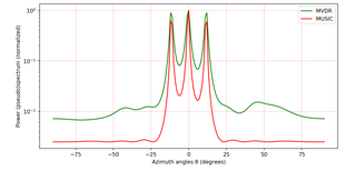
English: Spatial frequencies estimation (source code).
Русский: Оценка пространтвенных частот (исходный код). |
| Date | |
| Source | Own work |
| Author | Kirlf |
| PNG development | This plot was created with Matplotlib. |
| Source code | Python code"""
Developed by Vladimir Fadeev
(https://github.com/kirlf)
Kazan, 2017 / 2020
Python 3.7
"""
import numpy as np
import matplotlib.pyplot as plt
"""
Received signal model:
X = A*S + W
where
A = [a(theta_1) a(theta_2) ... a(theta_d)]
is the matrix of steering vectors
(dimension is M x d,
M is the number of sensors,
d is the number of signal sources),
A steering vector represents the set of phase delays
a plane wave experiences, evaluated at a set of array elements (antennas).
The phases are specified with respect to an arbitrary origin.
theta is Direction of Arrival (DoA),
S = 1/sqrt(2) * (X + iY)
is the transmit (modulation) symbols matrix
(dimension is d x T,
T is the number of snapshots)
(X + iY) is the complex values of the signal envelope,
W = sqrt(N0/2)*(G1 + jG2)
is additive noise matrix (AWGN)
(dimension is M x T),
N0 is the noise spectral density,
G1 and G2 are the random Gaussian distributed values.
"""
M = 10 # number of sensors
SNR = 10 # Signal-to-Noise ratio (dB)
d = 3 # number sources of EM waves
N = 50 # number of snapshots
""" Signal matrix """
S = ( np.sign(np.random.randn(d,N)) + 1j * np.sign(np.random.randn(d,N)) ) / np.sqrt(2) # QPSK
""" Noise matrix
Common formula:
AWGN = sqrt(N0/2)*(G1 + jG2),
where G1 and G2 - independent Gaussian processes.
Since Es(symbol energy) for QPSK is 1 W, noise spectral density:
N0 = (Es/N)^(-1) = SNR^(-1) [W] (let SNR = Es/N0);
or in logarithmic scale::
SNR_dB = 10log10(SNR) -> N0_dB = -10log10(SNR) = -SNR_dB [dB];
We have SNR in logarithmic (in dBs), convert to linear:
SNR = 10^(SNR_dB/10) -> sqrt(N0) = (10^(-SNR_dB/10))^(1/2) = 10^(-SNR_dB/20)
"""
W = ( np.random.randn(M,N) + 1j * np.random.randn(M,N) ) / np.sqrt(2) * 10**(-SNR/20) # AWGN
mu_R = 2*np.pi / M # standard beam width
resolution_cases = ((-1., 0, 1.), (-0.5, 0, 0.5), (-0.3, 0, 0.3)) # resolutions
for idxm, c in enumerate(resolution_cases):
""" DoA (spatial frequencies) """
mu_1 = c[0]*mu_R
mu_2 = c[1]*mu_R
mu_3 = c[2]*mu_R
""" Steering vectors """
a_1 = np.exp(1j*mu_1*np.arange(M))
a_2 = np.exp(1j*mu_2*np.arange(M))
a_3 = np.exp(1j*mu_3*np.arange(M))
A = (np.array([a_1, a_2, a_3])).T # steering matrix
""" Received signal """
X = np.dot(A,S) + W
""" Rxx """
R = np.dot(X,np.matrix(X).H)
U, Sigma, Vh = np.linalg.svd(X, full_matrices=True)
U_0 = U[:,d:] # noise sub-space
thetas = np.arange(-90,91)*(np.pi/180) # azimuths
mus = np.pi*np.sin(thetas) # spatial frequencies
a = np.empty((M, len(thetas)), dtype = complex)
for idx, mu in enumerate(mus):
a[:,idx] = np.exp(1j*mu*np.arange(M))
# MVDR:
S_MVDR = np.empty(len(thetas), dtype = complex)
for idx in range(np.shape(a)[1]):
a_idx = (a[:, idx]).reshape((M, 1))
S_MVDR[idx] = 1 / (np.dot(np.matrix(a_idx).H, np.dot(np.linalg.pinv(R),a_idx)))
# MUSIC:
S_MUSIC = np.empty(len(thetas), dtype = complex)
for idx in range(np.shape(a)[1]):
a_idx = (a[:, idx]).reshape((M, 1))
S_MUSIC[idx] = np.dot(np.matrix(a_idx).H,a_idx)\
/ (np.dot(np.matrix(a_idx).H, np.dot(U_0,np.dot(np.matrix(U_0).H,a_idx))))
plt.subplots(figsize=(10, 5), dpi=150)
plt.semilogy(thetas*(180/np.pi), np.real( (S_MVDR / max(S_MVDR))), color='green', label='MVDR')
plt.semilogy(thetas*(180/np.pi), np.real((S_MUSIC/ max(S_MUSIC))), color='red', label='MUSIC')
plt.grid(color='r', linestyle='-', linewidth=0.2)
plt.xlabel('Azimuth angles (degrees)')
plt.ylabel('Power (pseudo)spectrum (normalized)')
plt.legend()
plt.title('Case #'+str(idxm+1))
plt.show()
""" References
1. Haykin, Simon, and KJ Ray Liu. Handbook on array processing and sensor networks. Vol. 63. John Wiley & Sons, 2010. pp. 102-107
2. Hayes M. H. Statistical digital signal processing and modeling. – John Wiley & Sons, 2009.
3. Haykin, Simon S. Adaptive filter theory. Pearson Education India, 2008. pp. 422-427
4. Richmond, Christ D. "Capon algorithm mean-squared error threshold SNR prediction and probability of resolution." IEEE Transactions on Signal Processing 53.8 (2005): 2748-2764.
5. S. K. P. Gupta, MUSIC and improved MUSIC algorithm to esimate dorection of arrival, IEEE, 2015.
"""
|
Licensing
I, the copyright holder of this work, hereby publish it under the following license:
This file is licensed under the Creative Commons Attribution-Share Alike 4.0 International license.
- You are free:
- to share – to copy, distribute and transmit the work
- to remix – to adapt the work
- Under the following conditions:
- attribution – You must give appropriate credit, provide a link to the license, and indicate if changes were made. You may do so in any reasonable manner, but not in any way that suggests the licensor endorses you or your use.
- share alike – If you remix, transform, or build upon the material, you must distribute your contributions under the same or compatible license as the original.
File history
Click on a date/time to view the file as it appeared at that time.
| Date/Time | Thumbnail | Dimensions | User | Comment | |
|---|---|---|---|---|---|
| current | 05:41, 18 February 2019 | | 1,342 × 647 (112 KB) | Kirlf | User created page with UploadWizard |
File usage
The following pages on the English Wikipedia use this file (pages on other projects are not listed):
Global file usage
The following other wikis use this file:
- Usage on ca.wikipedia.org
- Usage on ru.wikipedia.org
- Usage on uk.wikipedia.org