
Size of this PNG preview of this SVG file: 800 × 416 pixels. Other resolutions: 320 × 166 pixels | 640 × 333 pixels | 1,024 × 532 pixels | 1,280 × 665 pixels | 2,560 × 1,331 pixels | 1,385 × 720 pixels.
Original file (SVG file, nominally 1,385 × 720 pixels, file size: 388 KB)
| This is a file from the Wikimedia Commons. Information from its description page there is shown below. Commons is a freely licensed media file repository. You can help. |
Summary
| Description |
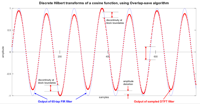
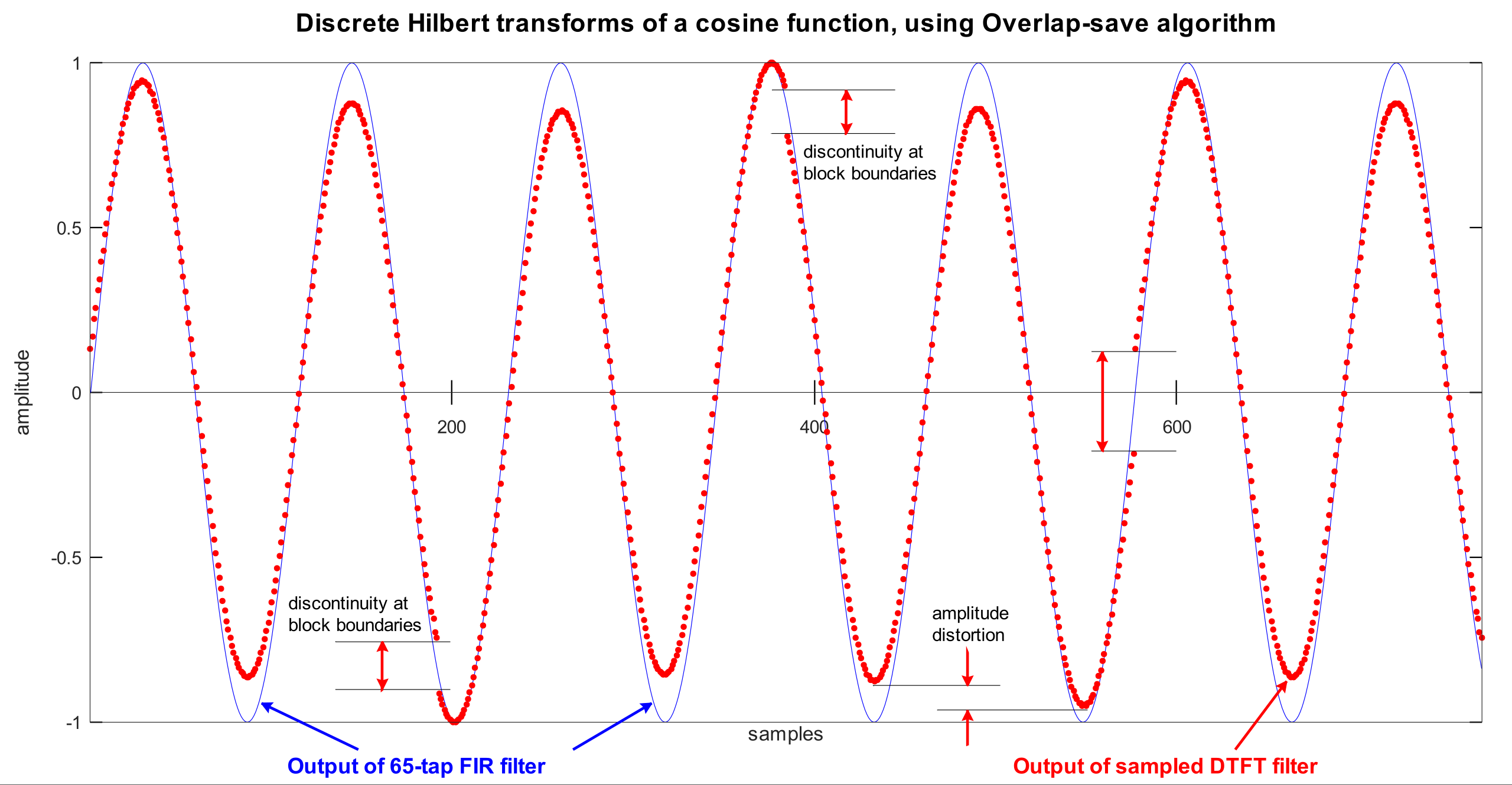
English: The blue graph shows a sine function that was created by computing the Discrete Hilbert transform of a cosine function. The cosine function was divided into 4 overlapping segments, which were individually convolved with an FIR Hilbert transform filter, and the 4 output segments were seamlessly pieced together. If the DFT of the FIR filter is replaced by the trivial samples of the DTFT of an IIR Hilbert transform filter, the cosine function segments are effectively convolved with a periodic summation of the IIR filter. That results in some frequency-dependent amplitude distortion and discontinuities at the segment boundaries. Examples of these effects are shown in the red graph. |
|||
| Date | ||||
| Source | Own work | |||
| Author | Bob K | |||
| Permission (Reusing this file) |
I, the copyright holder of this work, hereby publish it under the following license:
|
|||
| Other versions |
This file was derived from: Discrete Hilbert transforms of a cosine function, using piecewise convolution.jpg |
|||
| SVG development | This vector image was created with LibreOffice. |
|||
| Octave/gnuplot source | click to expand
This graphic was created with the help of the following Octave script: graphics_toolkit gnuplot
pkg load signal
clear all; close all; clc
hfig = figure("position",[100 200 1108 576]);
x1 = .06; % left margin for label
x2 = .02; % right margin
y1 = .08; % bottom margin for annotation
y2 = .08; % top margin for title
width = 1-x1-x2;
height= 1-y1-y2;
%=======================================================
subplot("position",[x1 y1 width height])
hold on
box on
set(gca, "xaxislocation","origin")
title("Discrete Hilbert transforms of a cosine function, using Overlap-save algorithm",...
"fontsize",14);
xlabel("samples");
ylabel("amplitude");
% Create a 64th-order Hilbert transform filter.
M = 65;
h = zeros(1,M);
n = -31:2:31;
h(33+n) = (2/pi)./n; % applies a rectangular window to the IIR function
% Derive overlap-save parameters. Note that our choice of M causes the FFT size (N)
% to be a power-of-2, which is efficient, but not necessary.
overlap = M-1;
N = 4*overlap; % an efficient block-size
step_size = N-overlap;
M2 = overlap/2; % length of the edge effects for a zero-phase (non-causal) filter
h = [h(1+M2:M) zeros(1,N-M) h(1:M2)]; % convert filter to zero-phase
H1 = fft(h); % transfer function
H2 = i*[0 -ones(1,N/2-1) ones(1,N/2)]; % or just sample the DTFT
% Create an input function
num_steps = 4; % signal length, in steps
n = (0 : num_steps*step_size+overlap)-M2; % sample indices (minus filter delay)
cycles_per_step = 5/3; % just a non-integer
cycles_per_sample = cycles_per_step / step_size;
x = cos(2*pi*cycles_per_sample*n); % transform a pure sinusoid
% Overlap-Save convolution
position = 0;
while position+N <= length(x)
yt = real(ifft( fft(x(position+(1:N)) ).* H1 ));
y1(position+(1:step_size)) = yt(1+M2 : N-M2);
% The next 2 lines are equivalent, so the 2nd one is commented out.
yt = real(ifft( fft(x(position+(1:N)) ).* H2 ));
% yt = imag(hilbert(x(position+(1:N))));
y2(position+(1:step_size)) = yt(1+M2 : N-M2);
position = position + step_size;
end
% Compare the results.
% Use unconnected dots for y2 to reveal the discontinuities at block boundaries.
y1 = y1 / max(abs(y1));
y2 = y2 / max(abs(y2));
plot(y1, "b");
plot(y2, "r."); % unconnected dots
xlim([1 length(y1)])
ylim([-1 1])
% Calling function annotation() changes the gnuplot cursor units to a normalized ([0,1])
% coordinate system, which is then used to obtain the coordinates used below.
annotation("textbox", [.19 .025 0 0], "fitboxtotext","on", "string",...
"Output of 65-tap FIR filter", "color","blue", "fontsize",12, "fontweight","bold")
annotation("textbox", [.67 .025 0 0], "fitboxtotext","on", "string",...
"Output of sampled DTFT filter","color","red", "fontsize",12, "fontweight","bold")
annotation("arrow", [.237 .173], [.045 .104],...
"headstyle","vback1", "headlength",5, "headwidth",5,...
"linewidth",2, "color","blue")
annotation("arrow", [.379 .431], [.045 .104],...
"headstyle","vback1", "headlength",5, "headwidth",5,...
"linewidth",2, "color","blue")
annotation("arrow", [.817 .851], [.045 .132],...
"headstyle","vback1", "headlength",5, "headwidth",5,...
"linewidth",2, "color","red")
%annotation("arrow", [.734 .717], [.045 .095],...
% "headstyle","vback1", "headlength",5, "headwidth",5,...
% "linewidth",2, "color","red")
% Annotate the three block boundaries
text(394, .7, {"discontinuity at";"block boundaries"})
text(110, -.67, {"discontinuity at";"block boundaries"})
annotation("line", [.222 .298], [.183 .183])
annotation("line", [.222 .298], [.122 .122])
annotation("doublearrow", [.253 .253], [.122 .183],...
"head1style","vback1", "head2style","vback1",...
"head1length",5, "head1width",5, "head2length",5, "head2width",5,...
"linewidth",2, "color","red")
annotation("line", [.511 .592], [.885 .885])
annotation("line", [.511 .592], [.830 .830])
annotation("doublearrow", [.560 .560], [.830 .885],...
"head1style","vback1", "head2style","vback1",...
"head1length",5, "head1width",5, "head2length",5, "head2width",5,...
"linewidth",2, "color","red")
annotation("line", [.722 .778], [.552 .552])
annotation("line", [.722 .778], [.425 .425])
annotation("doublearrow", [.729 .729], [.425 .552],...
"head1style","vback1", "head2style","vback1",...
"head1length",5, "head1width",5, "head2length",5, "head2width",5,...
"linewidth",2, "color","red")
% Annotate the amplitude distortion
text(465, -.7, {"amplitude";"distortion"})
annotation("line", [.578 .662], [.126 .126])
annotation("line", [.620 .719], [.095 .095])
annotation("arrow", [.640 .640], [.168 .126],...
"headstyle","vback1", "headlength",5, "headwidth",5,...
"linewidth",2, "color",red")
annotation("arrow", [.640 .640], [.050 .095],...
"headstyle","vback1", "headlength",5, "headwidth",5,...
"linewidth",2, "color","red")
% I actually used the export function on the GNUPlot figure toolbar.
print(hfig,"-dsvg", "-S1108,576","-color",...
'C:\Users\BobK\Discrete Hilbert transforms of a cosine function, using piecewise convolution.svg')
|
File history
Click on a date/time to view the file as it appeared at that time.
| Date/Time | Thumbnail | Dimensions | User | Comment | |
|---|---|---|---|---|---|
| current | 12:20, 28 May 2019 | | 1,385 × 720 (388 KB) | Bob K | Add another text() function annotation. |
| 03:46, 28 May 2019 |  | 1,385 × 720 (390 KB) | Bob K | User created page with UploadWizard |
File usage
The following pages on the English Wikipedia use this file (pages on other projects are not listed):